UNIT 4 : BIVARIATE STATISTICS
Key unit Competence: Extend understanding, analysis and interpretation
of bivariate data to correlation coefficients andregression lines
4.0 INTRODUCTORY ACTIVITY
In Kabeza village, after her 9 observations about farming,
UMULISA saw that in every house observed, where there is a cow (X) if
there is also domestic duck (Y), then she got the following results:
(1,4) ,( 2,8) , (3,4) , (4,12) , (5,10),(6,14) , (7,16) , (8,6 ), (9,18)
a. Represent this
information graphically in (x, y) − coordinates .
b. Find the equation of line joining any two points of the graph and guess the
name of this line.
c. According to your observation from (a), explain in your own words if there is any
relationship between the variation of Cows (X) and the variation of domestic duck (Y).
4.1 Bivariate data, scatter diagram and types of correlation
ACTIVITY 4.1
Consider the situation in which the mass, y (g), of a chemical is
related to the time , x minutes, for which the chemical reaction hasbeen taking place ,according to the table.
a) Plot the above information in (x, y) coordinates.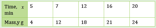
b) Explain in your own words the relationship between x and y
In statistics, bivariate or double series includes technique of analyzing data in
two variables, when focus on the relationship between a dependent variable-y
and an independent variable-x.
For example, between age and weight, weight and height, years of education
and salary, amount of daily exercise and cholesterol level, etc. As with data for a
single variable, we can describe bivariate data both graphically and numerically.
In both cases we will be primarily concerned with determining whether there
is a linear relationship between the two variables under consideration or not.
It should be kept in mind that a statistical relationship between two variables
does not necessarily imply a causal relationship between them. For example,
a strong relationship between weight and height does not imply that either
variable causes the other.
Scatter plots or Scatter diagram and types of correlation
Consider the following data which relate x, the respective number of branches
that 10 different banks have in a given common market, with y, the correspondingmarket share of total deposits held by the banks:
The scatter plot or scatter diagram (in the figure above) indicates that, roughly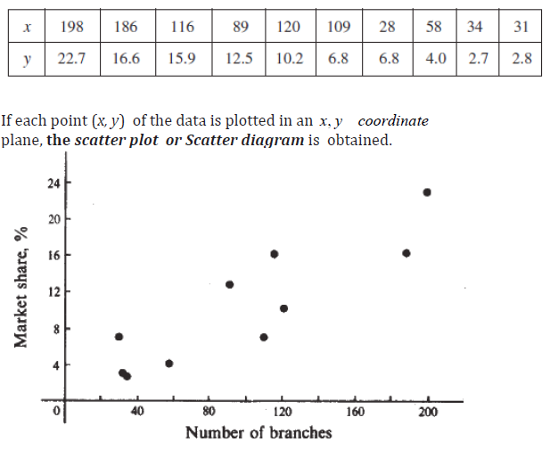
speaking, the market share increases as the number of branches increases. We
say that x and y have a positive correlation.
On the other hand, consider the data below, which relate average daily
temperature x, in degrees Fahrenheit, and daily natural gas consumption y, incubic metre.
Finally, consider the data items (x, y) below, which relate daily temperature x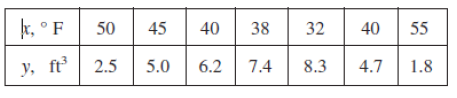
over a 10-day period to the Dow Jones stock average y.
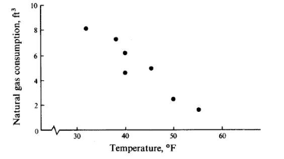
We see that y tends to decrease as x increases. Here, x and y have a negative
correlation.
Finally, consider the data items (x, y) below, which relate daily temperature x
over a 10-day period to the Dow Jones stock average y: (63, 3385); (72, 3330);
(76, 3325); (70, 3320); (71, 3330); (65, 3325); (70, 3280); (74, 3280) ;(68,3300); (61, 3265).
There is no apparent relationship between x and y (no correlation or Weak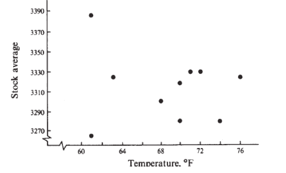
correlation.
APPLICATION ACTIVITY 4.1
One measure of personal fitness is the time taken for an individual’s
pulse rate to return to normal after strenuous exercise, the greater the
fitness, the shorter the time. Following a short program of strenuous
exercise Norman recorded his pulse rates P at time t minutes after
he had stopped exercising. Norman’s results are given in the tablebelow.
a) Draw a scatter diagram to represent this information in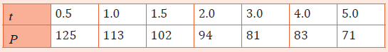
(x, y)coordinatesb) Explain the relationship between Norman’s pulse P and time t.
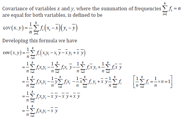
In case of two variables, say x and y, there is another important result called
covariance of x and y, denoted cov(x, y) .
The covariance of variables x and y is a measure of how these two variables
change together. If the greater values of one variable mainly correspond with the
greater values of the other variable, and the same holds for the smaller values,
i.e. the variables tend to show similar behavior, the covariance is positive. In
the opposite case, when the greater values of one variable mainly correspond
to the smaller values of the other, i.e. the variables tend to show opposite
behavior, the covariance is negative. If covariance is zero the variables are said
to be uncorrelated, itmeans that there is no linear relationship between them.
Therefore, the sign of covariance shows the tendency in the linear relationshipbetween the variables. The magnitude of covariance is not easy to interpret.
The Pearson’s coefficient of correlation (or Product moment coefficient of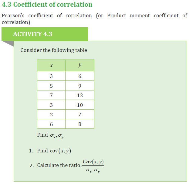
correlation or simply coefficient of correlation), denoted by r, is a measure ofthe strength of linear relationship between two variables.
Properties of the coefficient of correlation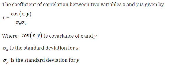
a) The coefficient of correlation does not change the measurement scale.
That is, if the height is expressed in meters or feet, the coefficient of
correlation does not change.
b) The sign of the coefficient of correlation is the same as the covariance.
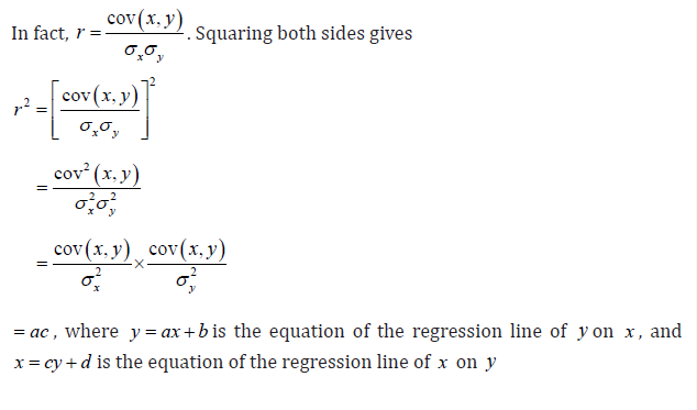
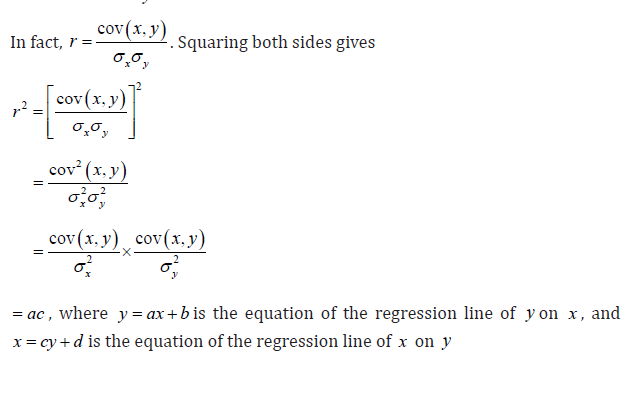
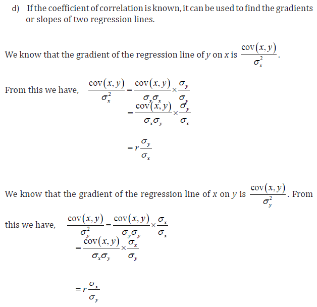
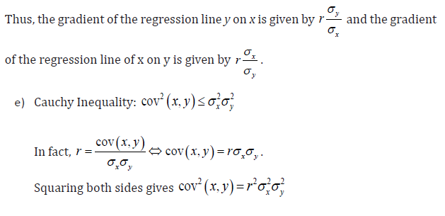
c) The square of the coefficient of correlation is equal to the product of the
gradient of the regression line of y on x , and the gradient of the regressionline of x on y .
g) If the linear coefficient of correlation takes values closer to −1, the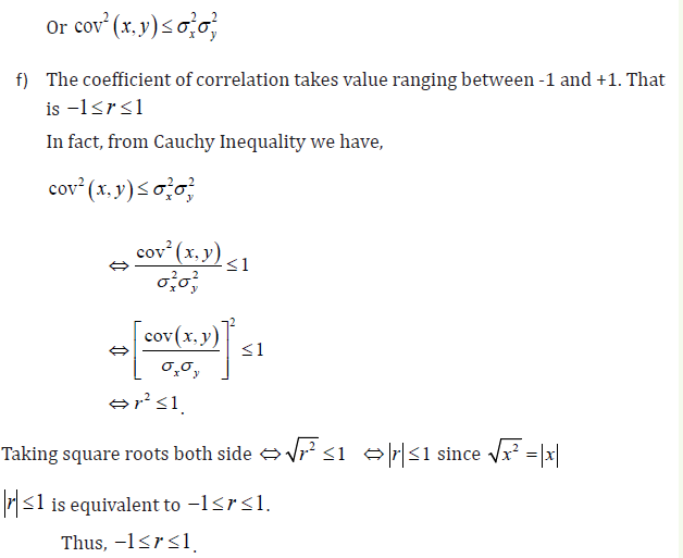
correlation is strong and negative, and will become stronger the closer
rapproaches −1.
h) If the linear coefficient of correlationtakes values close to 1 the correlation
is strong and positive, and will become stronger the closer r approaches 1
i) If the linear coefficient of correlationtakes values close to 0, the correlation is weak.
j) If r = 1or r = −1, there is perfect correlation and the line on the scatter
plot is increasing or decreasing respectively.k) If r = 0, there is no linear correlation.
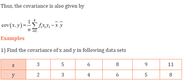
Examples:
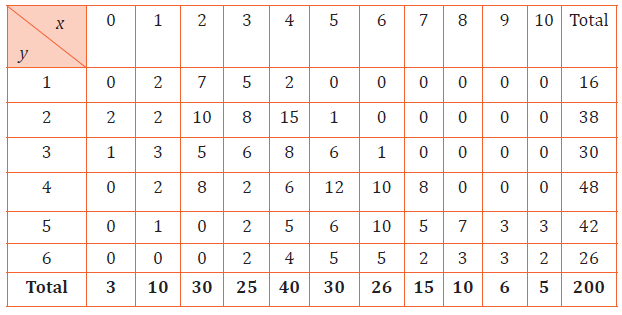
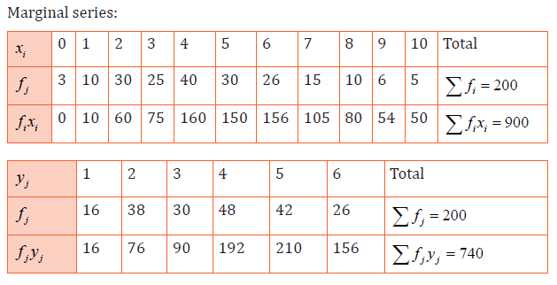
1) A test is made over 200 families on number of children (x) and number of
beds y per family. Results are collected in the table below
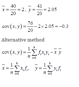
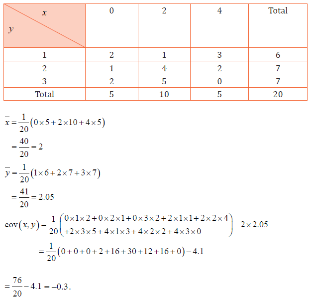
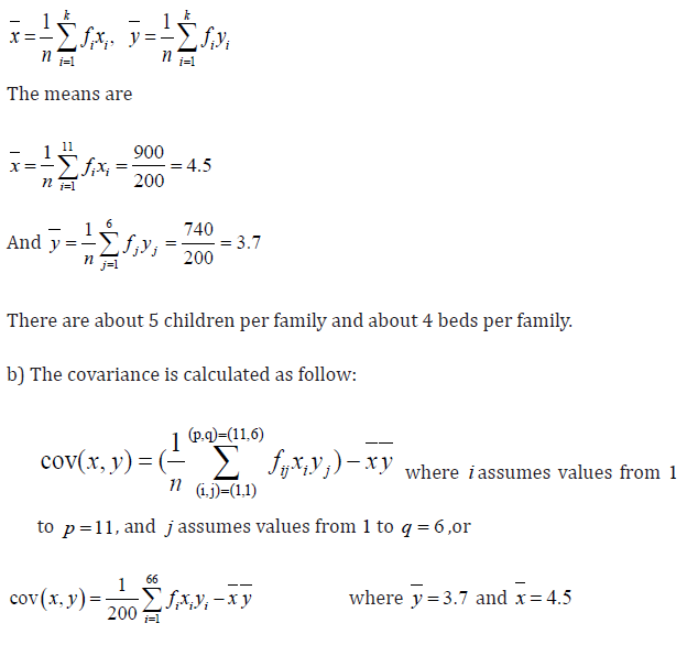
a) What is the average number for children and beds per a family?
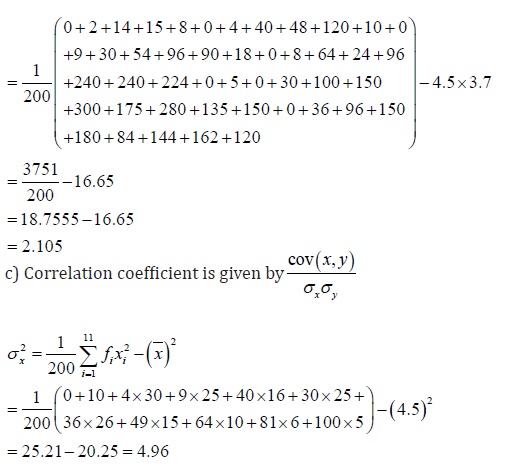
b) Find the covariance.
c) Can we confirm that there is a high linear correlation between the number of
children and number of beds per family?
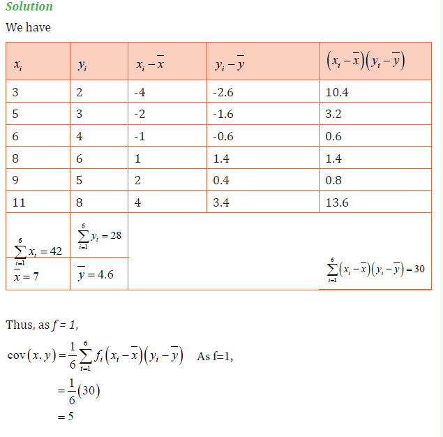
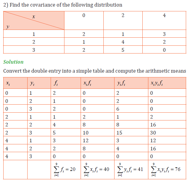
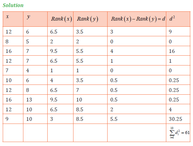
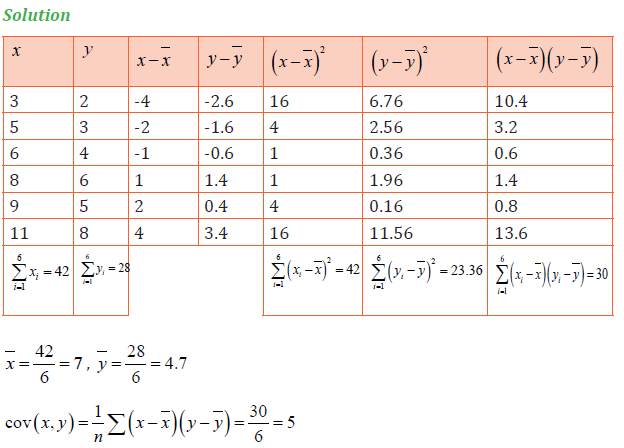
Solution
a) Average number of children per family:Contingency table:
Spearman’s coefficient of rank correlation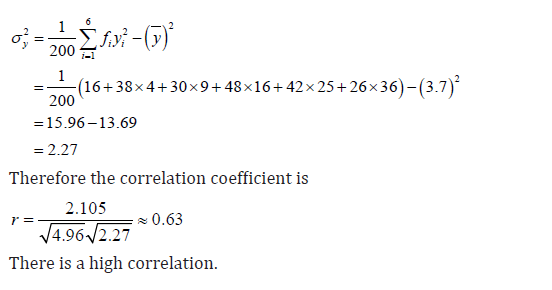
A Spearman coefficient of rank correlation or Spearman’s rho is measure
of statistical dependence between two variables. It assesses how well the
relationship between two variables can be described using a monotonic
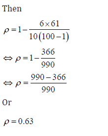
function. The Spearman’s coefficient of rank correlation is denoted and defined by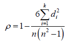
Where, d refers to the difference of ranks between paired items in two series and
n is the number of observations. It is much easier to calculate the Spearman’s
coefficient of rank correlation than to calculate the Pearson’s coefficient
of correlation as there is far less working involved. However, in general, the
Pearson’s coefficient of correlation is a more accurate measure of correlation
when data are numerical.
Method of ranking
Ranking can be done in ascending order or descending order.
Examples:
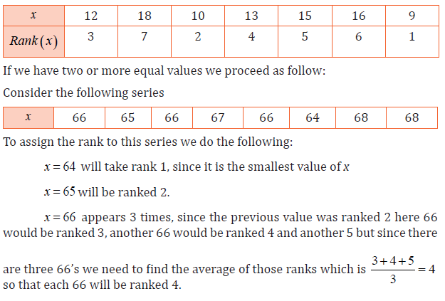
1) Suppose that we have the marks, x, of seven students in this order:
12, 18, 10, 13, 15, 16, 9
We assign the rank 1, 2, 3, 4, 5, 6, 7 such that the smallest value of x will be
ranked 1.That is
CONTENT SUMMARY
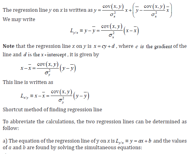
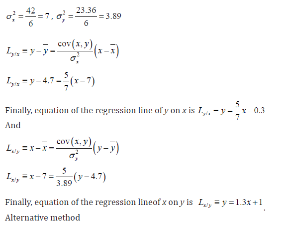
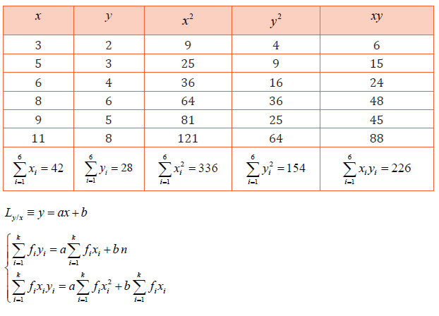
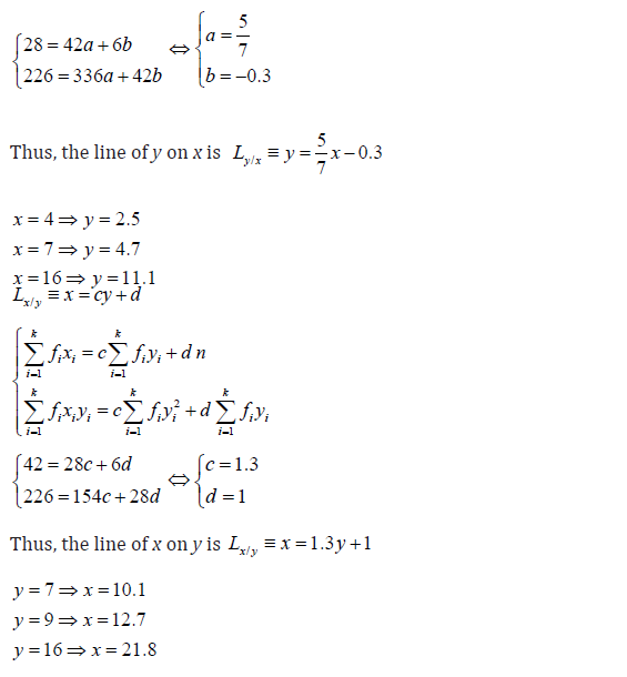
We use the regression line of y on x to predict a value of y for any given value
of x and vice versa, we use the regression line of x on y, to predict a value of
x for a given value of y. The “best” line would make the best predictions: the
observed y-values should stray as little as possible from the line. This straight
line is the regression line from which we can adjust its algebraic expressionsand it is written as y = ax + b , where a is the gradient and b is the y-intercept.
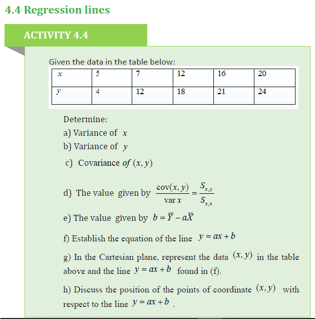
APPLICATION ACTIVITY 4.4
1. Consider the following table
4.5 Interpretation of statistical data (Application)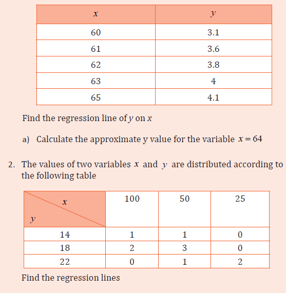
ACTIVITY 4.5Explain in your own words how statistics, especially bivariate
statistics, can be used in our daily life.
Bivariate statistics can help in prediction of a value for one variable if we know
the value of the other.
Examples:
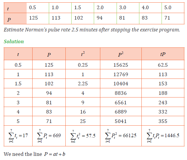
1. One measure of personal fitness is the time taken for an individual’s pulse
rate to return to normal after strenuous exercise, the greater the fitness, the
shorter the time. Following a short program of strenuous exercise Norman
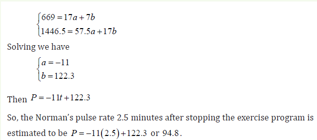
recorded his pulse rates P at time t minutes after he had stopped exercising.Norman’s results are given in the table below.
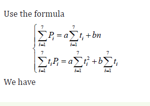
iv. State with a reason whether it is sensible to conclude from your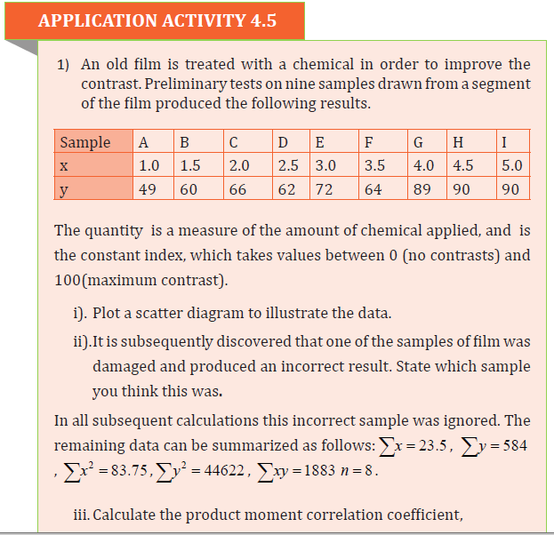
answer to part( iii) that and are linearly related.
v. The line of regression of on x has equation y = ax + b . Calculate the
value of a and b each correct to three significant figures.
vi. Use your regression line to estimate what the contrast index
corresponding to the damaged piece of film would have been if the
piece has been undamaged.
vii.State with a reason, whether it would be sensible to use your
regression equation to estimate the contrast index when the quantityof chemical applied to the film is zero.
4.6 END UNIT ASSESSMENT
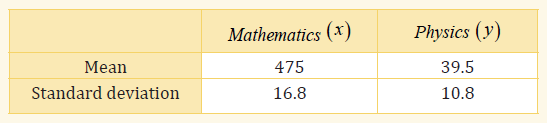
1) The following results were obtained from lineups in Mathematicsand Physics examinations:
4) The table below shows the marks awarded to six students in a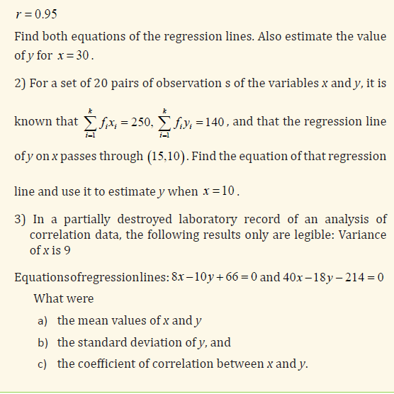
competition:
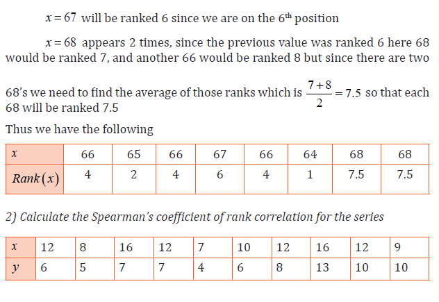
Calculate a coefficient of rank correlation.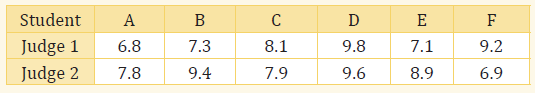
5) A company is to replace its fleet of cars. Eight possible models
are considered and the transport manager is asked to rank them,
from 1 to 8, in order of preference. A saleswoman is asked to use
each type of car for a week and grade them according to theirsuitability for the job (A-very suitable to E-unsuitable).
a. Calculate the Spearman’s coefficient of rank correlation between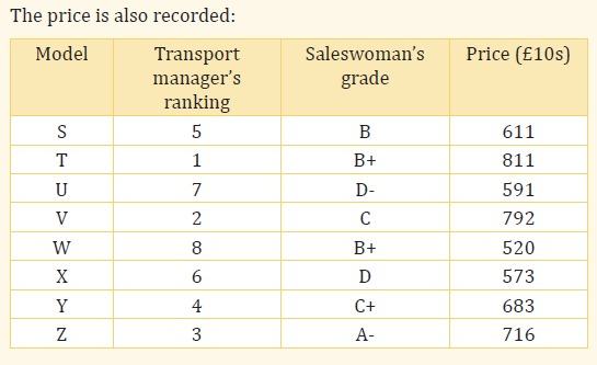
i. price and transport manager’s rankings,
ii. price and saleswoman’s grades.
b. Based on the result of a. state, giving a reason, whether it would
be necessary to use all three different methods of assessing the cars.
c. A new employee is asked to collect further data and to do some
calculations. He produces the following results:
The coefficient of correlationbetween
i. price and boot capacity is 1.2,
ii. maximum speed and fuel consumption in miles per
gallons is -0.7,
iii. price and engine capacity is -0.9
For each of his results say, giving a reason, whether you think
it is reasonable.
d. Suggest two sets of circumstances where Spearman’s coefficient
of rank correlation would be preferred to the Pearson’scoefficient of correlation as a measure of association.