ICT

Key Unit Competency: By the end of this unit, you should be able to: 

1. Work with spreadsheets and apply basic manipulation of cell content using arithmetic operations. 

Introduction

A spreadsheet program is an interactive program that enables the user to layout and organise numerical data tabular form. Spreadsheets contain rows and columns that intersect to form cells into which  data are entered. 

Examples of spreadsheet programs include the following: Microsoft (MS) Excel, Lotus 1-2-3, Quattro Pro, Multiplan, and Super Calc among others. The spreadsheet program discussed in this unit is Microsoft Excel 2013 (Ms Excel 2013). 

4.1 Definition and Role of a Spreadsheet 

A spreadsheet is a software that enables the user to organise numerical data on the screen in a tabular form. The program is made up of rows and columns used to present and analyse numerical data. 

The word spreadsheet is also used to describe an electronic document in which data is arranged in the rows and columns of a grid. A spreadsheet can be manipulated and used in calculations.

Spreadsheets enable the user to enter data, edit and perform calculations, as well as present data in graphic form. 

4.1.1 Features of Spreadsheets 

(a) They consist of a workbook and worksheets. 

(b) Every worksheet consists of cells where data is entered.  

(c) Every individual cell has a unique cell address used for identification. 

(d) It contains inbuilt formulas known as functions that enable the user to perform calculations quickly. 

(e) It allows presentation of information using charts. 

4.1.2 Create, Save, and Open a Workbook

A workbook refers to a file that can contain one or more worksheets used to organise different kinds of related data.  

A worksheet is a form containing cells that are organised in rows and columns. A worksheet on a computer screen resembles a sheet of paper with multiple columns that are used to analyse numerical data. 

Opening Microsoft Excel Program

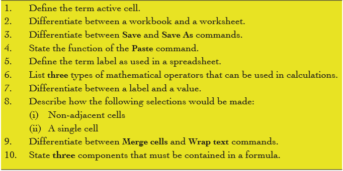
When you open Microsoft Excel 2013, the first window that is displayed is as shown in Figure 4.1 below:

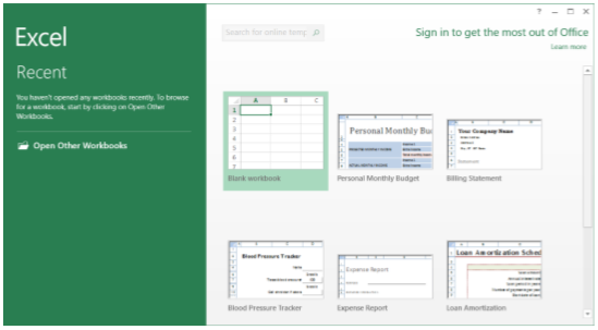
Figure 4.1: Opening Microsoft Excel 2013

There are four possible ways of starting Microsoft Excel program. These are: 

(i) Click START button, select All Apps then Click on Microsoft Office to display a list of programs contained in the office suite. Click on Excel 2013. 

(ii) Type the word RUN in the Search the web and Windows box next to the start button then press Enter key. Type excel in the dialog box that appears and click OK, or Press ENTER on the keyboard. 

(iii) Click START button then select Microsoft Excel 2013 if it was pinned on the start menu. 

(iv) Click Microsoft Excel 2013 icon if it was pinned on the task bar. 

Note: Any of the options above will display a window as shown in Figure 4.1. Click on the blank workbook icon to launch Excel and open a workbook window. 

Creating a workbook 

When Excel is launched, it automatically opens a workbook containing a worksheet with a default name of Sheet1. 

After the program is opened, the following steps can be used to create a new workbook: 

(i) Click on the File tab from the menu bar. 

(ii) Select New from the pull down menu. 

(iii) Click on the desired template from the right pane. For example, to create a new blank workbook, click on the Blank workbook option. 

Saving a workbook 

To save a workbook for the first time, do the following: 

(i) Click on the File Tab in the menu bar. 

(ii) Click the Save As option from the pull down menu that appears. The Save As window appears on the right as shown in Figure 4.2.

Figure 4.2: Saving a workbook 

(iii) Click on the location where the workbook is to be stored if it displayed on the Save As window. Otherwise click on Browse or Computer icon to display the Save As dialog box as shown in Figure 4.3. The keyboard shortcut for saving a document in Excel is as follows: Long press ALT then select F then A and finally press 1. 

(iv) Type the name of the workbook in the File name box. To select another storage location click on it on the left pane of the window.

(v) Click Save button.

 Once a workbook has been saved, a user can make changes to it and save it under the same name or a different name. To save changes on an existing workbook, do one of the following:

(i) Press Ctrl + S on the keyboard.

(ii) Click the File tab, then select Save command. 

(iii) Click the Save icon on the Quick Access Tool bar.

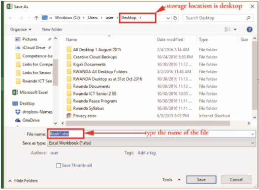
Figure 4.3: Choosing the location for saving a document 

To close an active workbook, do one of the following: 

(i) Click Close button on the title bar of the active worksheet. 

(ii) Press ALT + F4 on the keyboard. 

(iii) Click the File Tab then select Close command.

Opening an existing workbook 

It is also known as retrieving a saved workbook. To open an already saved workbook, do one of the following: 

It is also known as retrieving a saved workbook. To open an already saved workbook, do one of the following: 

(i) Click the File tab then select Open command. Select the location where the workbook was stored then click on the name of the workbook from the list displayed or click Browse to locate the file and finally click Open. 

(ii) If the file was among the ones that were recently created or modified, click on the File tab, select Open command then finally click on the name of the file in the Recent Workbooks pane .

(iii) Click Open icon on the Quick Access Toolbar. The open window appears. Proceed as in option (i) or (ii) above. 

(iv) Press CTRL + O on the keyboard and proceed as option (i) or (ii) above. 

(v) Open the location where the workbook was saved then double click on the workbook. 

4.2 Spreadsheet Environment 

The spreadsheet package used in this case is Microsoft Excel (Ms-excel) 2013. It contains the following parts: 

• Title bar: It displays the name of the application currently in use as well as the name of the active workbook. When a new spreadsheet is opened, Ms Excel allocates default names such as Book1, Book2 and so on. The default name changes any time the workbook is saved using a new name.

• Buttons: The title bar also contains three buttons which are: Minimise, Restore Down/Maximise and Close buttons at the top right corner. 

• Menu bar: This bar displays the following tabs: File, Home, Insert, Page Layout, Formulas, Data, Review and View. Additional tabs appear when a chart is inserted or selected. 

• Ribbon: The ribbon consists of icons of commands organised and classified into groups. Clicking on any tab on the menu bar displays a ribbon unique to it. For example, clicking on Page Layout tab displays a ribbon with 5 groups namely Themes, Page Setup, Scale to Fit, Sheet Options and Arrange. 

• The Quick Access Toolbar: It is a small customisable toolbar of the most commonly used commands located at the top left corner of the workbook window. By default, this bar contains Save, Undo and Redo commands. See Figure 4.4 on page 100.

It can be customised in the following ways:

(i) It can be made to appear above or below the ribbon. 

(ii) Commands can be added or removed from it. 

• Scroll bar: The scroll bar allows one to move or navigate through a large worksheet. There are two types of scroll bars the vertical scroll bar and horizontal scroll bar. Vertical scroll bar allows upward or downward movement on the worksheet while horizontal scroll bar allows movement from left to right and vice versa.

• Formula bar:  It provides the user with a box for entering or editing data or formula in a cell. It is located below the ribbon by default. It contains the cell naming box and the formula box used for entering a formula or editing data. 

Figure 4.4: Customising the Quick Access Toolbar

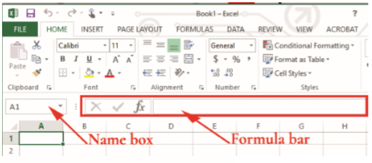
Figure 4.5: The formula bar contains the name box and the formula box 

• Status bar: It is located at the bottom of the window and it displays status on options that are selected to appear on the status bar. For example, to display average, count, or sum of selected cells is looking at the status bar. Figure 4.6 shows a display of the status bar.

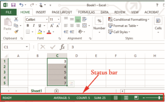
Figure 4.6: The Status Bar 

• Cell: It is an intersection of a row and a column where data is entered. 

• Active cell: It is also referred to as cell pointer or selected cell. It is a rectangular box highlighting the cell being worked with and where data is being entered. By default A1 is usually the active cell. To make a cell active simply click on it.

• Name box: It displays the name of the active cell. 

• Column Title: It is also known as column heading and is labelled in letters. This is a row containing the column labels. 

• Sheet Tab: It contains the name of the worksheets in the workbook. 

• Row Title: It is also known as row heading and is labelled in numbers. This is a column containing the row labels. 

Parts of the Microsoft Excel Window 

Figure 4.5 shows the parts of Microsoft Excel window.

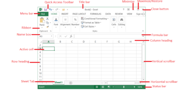
Figure 4.7: The Microsoft-Excel application window

4.3 Cell, Row, and Column basics

4.3.1 Definitions 

• Row: It is a range of horizontal cells having a unique number. They run vertically on the left side of the worksheet. 

• Column: It is a range of vertical cells labelled using a unique letter. They run horizontally at the top of the worksheet. 

4.3.2 Cell Content 

In this section we will discuss the different types of data in a cell. These types include: Labels, Values, Functions and Formulas. 

(a) Labels 

They are text or alphanumeric characters that are entered in a cell which cannot be manipulated mathematically. By default, all labels are aligned to the left of a cell.

Entering a Label 

(i) Click on the cell where the text is to be entered. 

(ii) Type the text. 

(iii) Press the Enter key or click on a different cell.

 (b) Values 

They are numeric data that can be manipulated mathematically. They include numbers, dates, time and currency among others. A value can be entered as a label if it is preceded by an apostrophe. By default, all values are aligned to the right of a cell.

 Entering Values 

(i) Click on the cell where the value is to be entered. 

(ii) Type the value. 

(iii) Press the Enter key or click on a different cell. 

(c) Formulas (or Formulae) 

They are mathematical expressions created by the user. Every formula must have the following components: 

(i) Begin with an equal sign (=). 

(ii) Contain mathematical operation such as +, -, / and *. 

(iii) Cell addresses that contain values. 

(d) Function 

They are in-built formulas in Excel. In-built means that they exist as essential parts of the program that the user can quickly apply to a cell in order to perform mathematical calculations. Every function must have the following components: 

(i) Begin with an equals sign (=). 

(ii) The name of the Function. 

(iii) The cell addresses that contain values. 

Entering formula Formulae can be typed within a cell in a worksheet but when the enter key is pressed, the actual cell displays the result of the calculation. 

To view the formulae, simply click on the cell, it will be automatically displayed on the formula bar. 

Enter data in a cell When data is typed in a cell, it is displayed in the selected cell as well as in the formula bar.  The data enters the cell when the Enter key or Arrow key is pressed.  Text can be wrapped on a cell by pressing ALT+ Enter while typing.

Selecting data 

This refers to highlighting a cell containing data that is supposed to be formatted. The table below summarises the different ways of selecting data in a worksheet.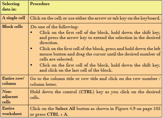


Copy and paste 

Copying is the process of creating a duplicate of data. The content remains in its original location as a copy of it is stored on the clipboard. A clipboard is a temporary storage location for items to be moved or copied. Pasting is the process of inserting the current clipboard content to a new location. To copy and paste, do the following:
 

(i) Select or highlight the data. 

(ii) Use one of the following options: 

• Right-click on the highlighted data then select Copy from the pop-up menu. Press Ctrl + C on the keyboard. From Home tab, click Copy icon under the Clipboard group. Figure 4.10 on page 103 shows a section of the Home tab ribbon showing the clipboard group. 

• The keyboard shortcut is as follows: Long press ALT then H and finally C key.

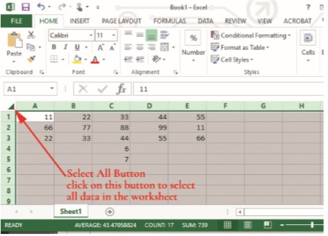
Figure 4.9: Using the Select All Data button

 

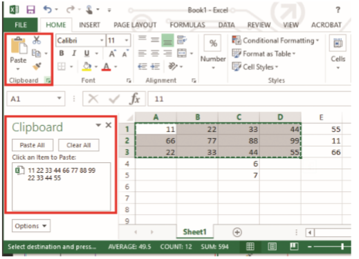
Figure 4.10: Copying and pasting

(iii) Position the cursor where the duplicate is to be placed. 

(iv) Paste it by doing one of the following: 

• From Home tab, click Paste icon under the Clipboard group. 

• Right-click at the cursor position and select Paste from the pop-up menu that appears. 

• Press Ctrl+ V on the keyboard. 

Copying can also be done using Format Painter command. This method is used when copying formats which had been previously applied on a cell or a group of cells. To copy formats do the following: 

(i) Select the cells containing the format to copy. 

(ii) Click Format Painter from clipboard group in the Home tab. 

(iii) Click the cells where the format is to be copied. 

Note: To copy the formatting in the selected cell or range to several locations, double-click the Format Painter button. Click on the first location to apply the format then the second, third all the way to the last one.

Figure 4.11: Using the Format Painter

Cut and paste 

Cutting is also known as moving. It is the process of changing the position of data to a new location. The data is deleted from its original location. 

To move data, do the following:

(i) Select or highlight the text or object. 

(ii) Use one of the following options: 

• From Home tab, click Cut icon under the Clipboard group. 

• Right-click on the highlighted text or object then select Copy from the pop-up menu. 

• Press Ctrl + X on the keyboard. 

(iii) Position the cursor where the data is to be transferred. 

(iv) Paste it by doing one of the following options:

• From Home tab, click Paste icon under the Clipboard group. 

• Right-click at the cursor position and select Paste from the pop-up menu that appears. 

• Press Ctrl + V on the keyboard. 

Changing row height 

The row height can be made smaller or larger than the default. There are two methods of changing a row height. 

Alternative 1 

(i) Place the mouse pointer at the boundary between two rows on the row title.  

(ii) When the mouse pointer changes to a two headed arrow, click and drag to the desired direction. 

(iii) Release the mouse button to apply. 

Alternative 2

(i) From Home tab, on the Cells group click on Format. A drop down menu appears as shown in Figure 4.12. keyboard shortcut is: Long press ALT key, then H followed by O to display a drop down menu.

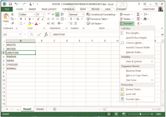
Figure 4.12: Changing the row height 

(ii) From the resulting menu select Row Height… A dialog box appears as shown in Figure 4.13. 

(iii) Type the desired value in the Row height box. 

(iv) Click OK.

Figure 4.13: Row Height dialog box

Changing column width 

The column width can be made narrow or wider than the default. There are two methods of changing a column width. 

Alternative 1 

(i) Place the mouse pointer at the boundary between two columns in the column title. 

(ii) When the mouse pointer changes to a two headed arrow, click and drag to the desired column width. 

(iii) Release the mouse button to apply.

Alternative 2 

(i) From Home tab, on the Cells group click on Format. 

(ii) From the resulting menu select Column Width… A dialog box appears as shown in Figure 4.14.

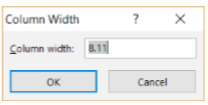
Figure 4.14: Column width dialog box. 

(iii) Type the desired value in the Column Width box. Click OK. 

Wrap text

Wrap text feature enables a cell to contain content that is larger than its size and all the content is displayed in multiple lines. The cell is automatically enlarged as data is entered. To wrap text, do the following: 

(i) Select the cell(s). 

(ii) Click on the Home tab then select Wrap text icon in the Alignment group. 

Alternatively 

(i) Select the cell(s). 

(ii) Click on the Home tab then select Format icon under the cells group. (iii) Click on Format Cells… from the drop down menu. The format cells dialog box appears as shown in Figure 4.15. The keyboard shortcut is: Long press ALT key, then H followed by O and finally E. 

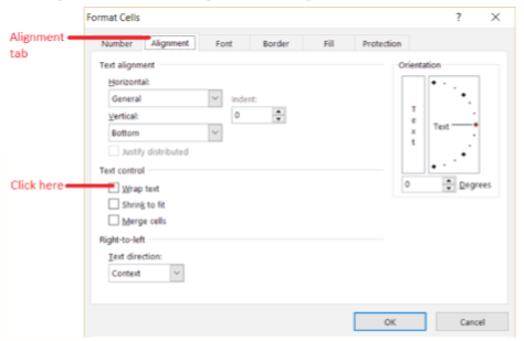
Figure 4.15: Wrapping text 

(iv) Click on the Wrap text under the Text control section. 

(v) Click OK to apply and close the dialog box. Figure 4.16 shows how the wrapped text will appear in the cell.

Figure 4.16: Cells containing wrapped text

Merge cells 

Merge cells refers to the combination of two or more horizontally or vertically adjacent cells to become one large cell that is displayed across multiple columns or rows.

The content of the first highlighted cell appears in the merged cell. A single cell that is created by combining two or more selected cells.

The cell reference for a merged cell is the upper-left cell in the original selected range.  To merge cells, do the following:
(i) Select the cells to be merged.
(ii) Click on the Home tab then select Merge & Center icon in the Alignment group. The cells are automatically merged. Figure 4.17 shows how the merged cells will appear.

Figure 4.17: Cells that have been merged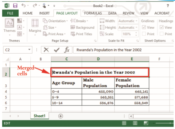 

Inserting a column or a row

It is possible to insert a row or a column between existing rows or columns respectively.To insert a row or a column, do the following:

Inserting a column

(i) Click on the column heading to select it.
(ii) Right-click on the selected column, and then click Insert from the resulting pop-up menu to automatically add a new column to the left of the selected column.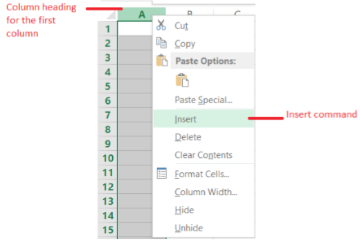 

 Figure 4.18: Click insert to add a column to the left 

Inserting a Row 

(i) Click on the row heading to select it. 

(ii) Right-click on the selected row, and then click Insert from the resulting popup menu to automatically add a new row above the selected row.

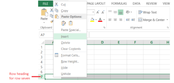
Figure 4.19: Click insert to add a row above row seven

 Deleting rows and columns

To delete rows or columns in a worksheet do the following: 

(i) Highlight a cell or cells to be deleted. 

(ii) Right-click on the selected cell(s) then select Delete… option from the pop-up. A dialog box appears as shown in Figure 4.20. 

(iii)  Select on Entire row option to delete the selected row(s) or Entire column option to delete the selected column(s). 

(iv) Click OK to apply.

Figure 4.20: Delete dialog box

Moving rows and columns 

To move a row or column in a worksheet, do the following: 

(i) Select the row or column to be moved. 

(ii) Move the mouse pointer to the edge of the selection until it changes from a regular cross to a four-sided arrow cursor. 

(iii) Then drag the column or row to a new location. 

(iv) Release the mouse button to place the row or column to its new location. 

Hide and unhide row/columns 

This feature is used to temporarily hide rows and columns from view in order to prevent certain data from being changed or deleted. It is also used to simplify the appearance of a spreadsheet. To hide or unhide a row or a column; do the following:

(i) From Home tab, on the Cells group click on Format. 

(ii) From the resulting drop down menu, point to Hide & Unhide then select the desired option from the side kick menu as shown in Figure 4.21 on page 112. The keyboard shortcut is: Long press ALT key, then H followed by O and finally U.

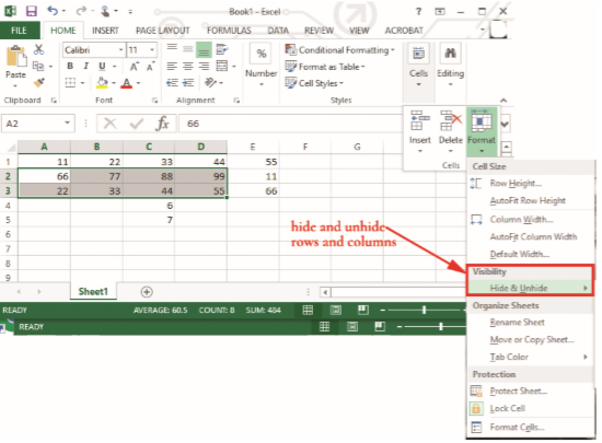
Figure 4.21: Hiding and unhiding columns

4.4 Formatting a Cell 

Formatting is the process of improving the appearance of a data in a worksheet. The following are some of the formatting options available in Microsoft Excel: font, text alignment and orientation, cell borders and fill colours, and formatting numbers and text. 

4.4.1 Font 

There are different ways of changing the font of text in a worksheet: 

(a) Using icons in the Home tab ribbon. 

To format font in cells using this option, do the following: 

(i) Select the cells. 

(ii) Click on the arrow on the Font list box as shown in Figure 4.22. 

(iii) Select the font from the list.

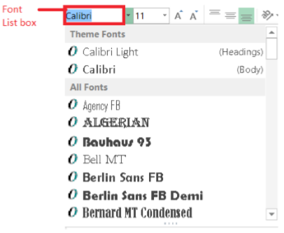
 Figure 4.22: The font list box

(b) Using the dialog box launcher 

(i) Select the cells to apply the format and do the following: 

(ii) From Home tab, under the Font group, click on the dialog box launcher to get a dialog box as shown in Figure 4.23. 

(iii) Select the desired font attributes. 

(iv) Click OK to apply. The keyboard shortcut is: Long press ALT key, then H followed by FN. Use the arrow keys to select a tab.

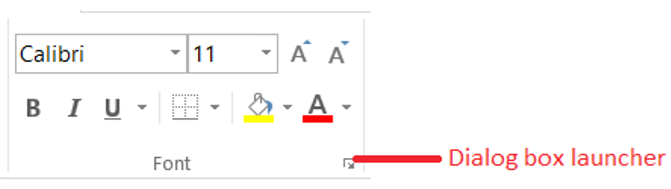
Figure 4.23: Using the dialog box launcher to change font

Figure 4.24: Selecting font attributes

4.4.2 Text Alignment and Orientation 

To format text alignment, do the following: 

(i) Select the cells to apply the format. 

(ii) From Home tab, under the Alignment group, click on the dialog box launcher. 

(iii) Select the desired alignment option from the available options in the resulting dialog box shown in Figure 4.25. 

(iv) Click OK to apply. The available options include: 

• Alignment: This contains the following options: 

• Text Alignment: It contains three options, namely horizontal, vertical and indent. 

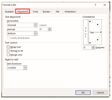
Figure 4.25: Controlling and aligning text

1.  Horizontal: It is used for changing the horizontal alignment of cell contents. Click on the box to make the desired option. 
2. Vertical: Used for changing the vertical alignment of cell contents. Click on the box to make the desired option. 
3.  Indent: It indents cell contents from any edge of the cell, depending on the selection made under Horizontal or Vertical options. 

• Orientation: Used to change the angle at which the text is inclined in the selected cells.

 Degrees: Sets the value in which text will be rotated in the selected cell. 

• Text control: The options under Text control are used to adjust how the text should appear in a cell. They include:

Wrap text: Wraps text into multiple lines in a  cell. The number of wrapped lines is dependent on the width of the column and the length of the cell contents. 
Shrink to fit: Decreases the apparent size of font characters so that all data in a selected cell fits within the column.
Merge cells: Joins two or more selected cells into one large cell. 

• Right-to-left: Select an option in the Text direction box to specify reading order and alignment.
• The keyboard shortcut is: Long press ALT key, then H followed by FN. Use the arrow keys to select a tab. 

4.4.3 Cell Borders 

The worksheet gridlines do not appear when a worksheet page is printed. The cell border helps in ensuring that the cell outline appears in the print out. They are also used for enhancing the appearance of a document. To apply cell borders, do the following: 

(i) Select the cells to apply the format. 

(ii) From Home tab, under the Font group click on dialog box launcher. 

(iii) Click on Border tab. A dialog box will appears as shown in Figure 4.26. 

(iv) Select the desired border style under Style option. 

(v) Click the buttons under Presets or Border to apply borders to the selected cells. To remove all borders, click the None button. It is also possible to click areas in the text box to add or remove borders. To change Colour, click on the Colour list box and select the desired colour from the colour palette. 

(vi) Click OK to apply. 

The keyboard shortcut is: Long press ALT key, then H followed by FN. Use the arrow keys to select a tab.

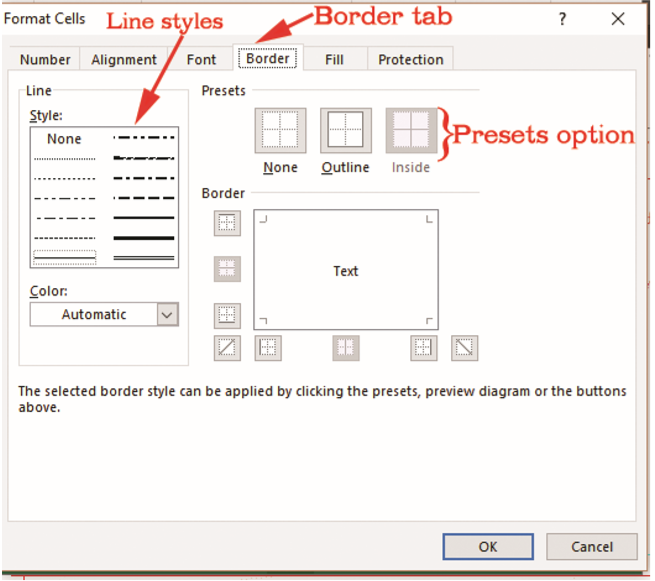
Figure 4.26: Formatting cell borders

4.4.4 Fill Colours 

To apply the fill colour command, do the following: 

(i) Select the cells to apply the format. 

(ii) From Home tab, under the Font group click on dialog box launcher. 

(iii) Click on Fill tab. A dialog box will appear as shown in Figure 4.27. 

(iv) Select the desired fill style from the available options, namely background colour, pattern colour, and pattern style and fill effects. 

(v) Click OK to apply. 

The keyboard shortcut is: Long press ALT key, then H followed by FN. Use the arrow keys to select a tab.

Figure 4.27: Formatting colours 

4.4.5 Formatting Number 

Select the cells to apply the format and do the following: 

(i) From Home tab, under the Font group click on dialog box launcher. 

(ii) Click on Number tab. A dialog box will appear as shown in Figure 4.28. The keyboard shortcut is: Long press ALT key, then H and finally FN.

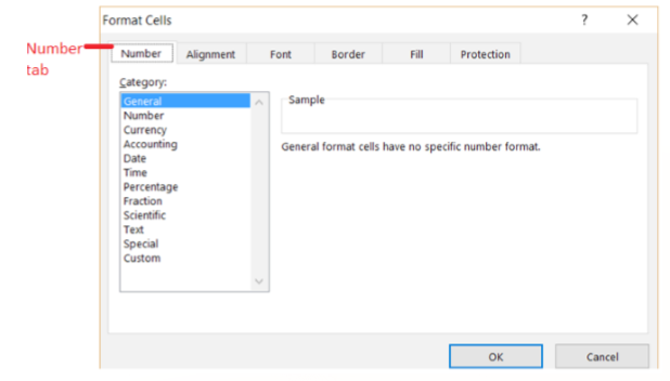
Figure 4.28: Formatting number

(iii) Under Category section, select an option and then select the desired options to specify a number format. The chosen format is shown as it will appear in the Sample box. 

(iv) Click OK to apply. 

4.5 Worksheet Basics

When excel is activated, a workbook is launched with a default worksheet. The user can insert, delete, rename, copy move a worksheet. The following commands can be used when manipulating a worksheet. 

4.5.1 Inserting a Worksheet

This feature enables the user to add a worksheet in a workbook. By default, the workbook in Microsoft Excel 2013 only comes along with one worksheet. To add another worksheet, do the following: 

(i) Right-click on the name of the sheet. A pull-up menu appears as shown in Figure 4.29.

Figure 4.29: Adding a worksheet 

(ii) Select Insert option. A dialog box appears as shown in Figure 4.30. 

(iii) Click OK to apply. The new worksheet name appears before the current worksheet.

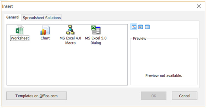
Figure 4.30: Inserting a worksheet 

This option is used when the entire worksheet is to be deleted. Do the following: 

(i) Right-click on the name of the sheet. A pull-up menu appears as shown in Figure 4.31. 

(ii) Select Delete option. The sheet is automatically deleted.

Figure 4.31: Click on Worksheet name then select Delete to apply

4.5.3 Renaming a Worksheet 

Renaming is the process of assigning a worksheet a different name. To rename a worksheet, do the following; 

(i) Double click on the name of the worksheet. The worksheet is highlighted as shown in Figure 4.32.

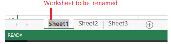
Figure 4.32: Renaming a worksheet

(ii) Type the desired name and then press Enter.

4.5.4 Copying and Moving a worksheet 

(i) Right-click on the name of the sheet. A pull-up menu appears as shown in Figure 4.33.

 

Figure 4.33: Moving or copying a worksheet

(ii) Select Move or Copy option. A dialog box appears as shown in Figure 4.34.

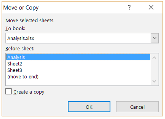
Figure 4.34: Moving a selected worksheet 

(iii) Select the book name in the To book: list and the worksheet to appear before it in the Before sheet: box. 

(iv) When Copying click on the Create a copy check box to enable it duplicate the worksheet else it will be moved. 

(v) Click OK to apply.

4.5.5 Grouping and Ungrouping Worksheets 

Grouping worksheets 

(i) Select the first worksheet to be included in the group. 

(ii) Press and hold the CTRL key on your keyboard. 

(iii) Select the next worksheet needed in the group. 

(iv) Release the CTRL key. 

(v) Select Group.

Ungrouping worksheets 

(i) Select the grouped worksheets to be ungrouped into separate worksheets. 

(ii) Select Ungroup.

4.6 Mathematical Operators 

Operators are symbols used in a formula to define the relationship between two or more values or cell references. They are symbols or signs that represent arithmetic operations in Excel formula. There are four major mathematical operators that can be used to write an expression. 

Figure 4.35 shows different operators as well as their functions. 

Figure 4.35:  Mathematical operators and their functions 

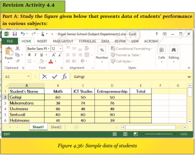
Figure 4.36 shows data about student’s marks of different subjects entered in a worksheet.

4.7 Definition of Key Words in this Unit

Revision Exercise 4