Topic outline
General
- S6: Subsidiary Maths SB File Uploaded 10/08/22, 18:32
- S6: Subsidiary Maths TG File Uploaded 10/08/22, 18:34
UNIT1: COMPLEX NUMBERS
Key unit competence
Perform operations on complex numbers in different forms and use them to solve related problems in Physics, Engeneering, etc.
Introductory activity

1. 1 Algebraic form of Complex numbers and their geometric representation
1.1.1 Definition of complex number


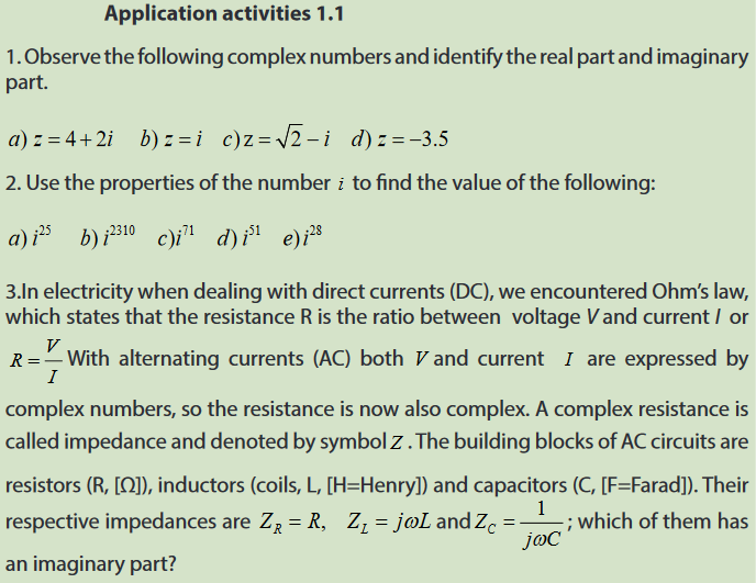
 Complex numbers are commonly used in electrical engineering, as well as in physics as it is developed in the last topic of this unit. To avoid the confusion between irepresenting the current andi for the imaginary unit, physicists prefer to use j to represent the imaginary unit.As an example , the Figure 1.1 below shows a simple current divider made up of a capacitor and a resistor. Using the formula, the current in the resistor is given by
 The product τ = CR is known as the time constant of the circuit, and the frequency for which1CRω= is called the corner frequency of the circuit. Because the capacitor has zero impedance at high frequencies and infinite impedance at low frequencies, the current in the resistor remains at its DC value TI for frequencies up to the corner frequency, whereupon it drops toward zero for higher frequencies as the capacitor effectively short-circuits the resistor. In other words, the current divider is a low pass filter for current in the resistor.Properties of the imaginary number “i”


 1.1.2 Geometric representation of a complex number
 The complex plane consists of two number lines that intersect in a right angle at the point (0,0) . The horizontal number line (known as x axis− in Cartesian plane) is the real axis while the vertical number line (the y axis− in Cartesian plane) is the imaginary axis.
 Complex impedances in seriesIn electrical engineering, the treatment of resistors, capacitors, and inductors can be unified by introducing imaginary, frequency-dependent resistances for the latter two (capacitor and inductor) and combining all three in a single complex number called the impedance.If you work much with engineers, or if you plan to become one, you’ll get familiar with the RC (Resistor-Capacitor) plane, just as you will with the RL (Resistor-Inductor) plane.Each component (resistor, an inductor or a capacitor) has an impedance that can be represented as a vector in the RX plane. The vectors for resistors are constant regardless of the frequency.
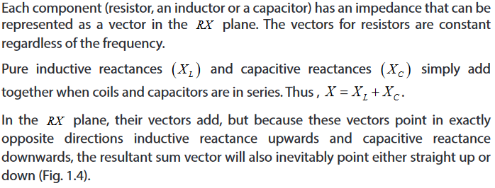

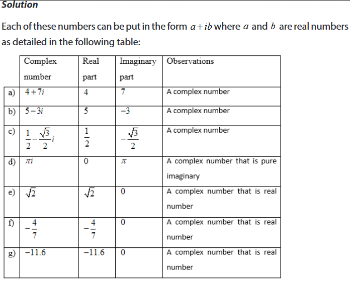
 Solutiona)

 1.1.3 Operation on complex numbers1.1.3.1 Addition and subtraction in the set of complex numbers
 Complex numbers can be manipulated just like real numbers but using the property
 whenever appropriate. Many of the definitions and rules for doing this are simply common sense, and here we just summarise the main definitions.
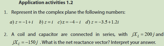
 Adding impedance vectorsIf you plan to become an engineer, you will need to practice adding and subtracting complex numbers. But it is not difficult once you get used to it by doing a few sample problems. In an alternating current series circuit containing a coil and capacitor, there is resistance, as well as reactance.Whenever the resistance in a series circuit is significant, the impedance vectors no longer point straight up and straight down. Instead, they run off towards the “northeast” (for the inductive part of the circuit) and “southeast” (for the capacitive part). This is illustrated in Figure 1.5.


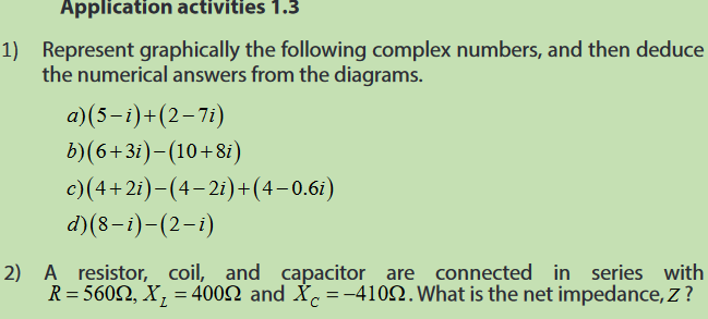
 In calculating a vector sum using the arithmetic method the resistance and reactance components add separately. The reactances 1Xand 2X might both be inductive (positive); they might both be capacitive (negative); or one might be inductive and the other capacitive.When a coil, capacitor, and resistor are connected in series (Figure 1.7), the resistance R can be thought of as all belonging to the coil, when you use the above formulae. (Thinking of it all as belonging to the capacitor will also work.)

 1.1.3.2 Conjugate of a complex number
 Every complex number z a bi= + has a corresponding complex number z−called conjugate of zsuch that z a bi−= − and affix of z is the “reflection” of affix of z about the real axis as illustrated in Figure 1.8.
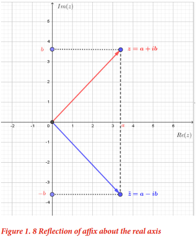

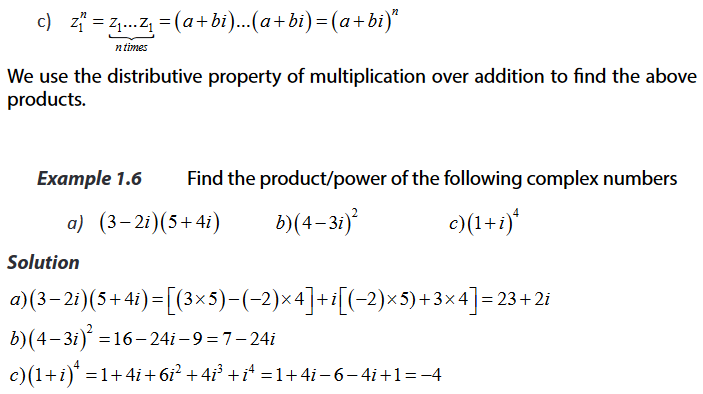
 1.1.3.3 Multiplication and powers of complex number
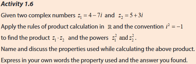

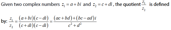
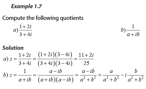
 1.1.3.4 Division in the set of complex numbers
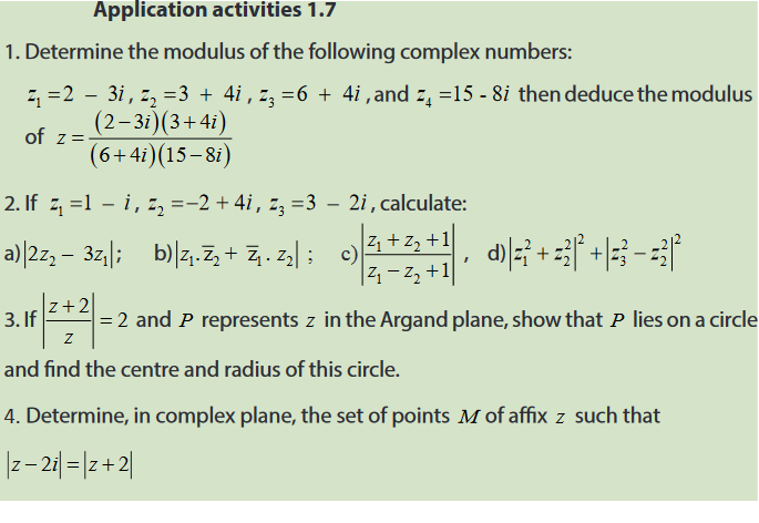
 1.1.4 Modulus of a complex number


 1.1.5 Square root of a complex number


 1.1.6 Equations in the set of complex numbers1.1.6.1 Simple linear equations of the form

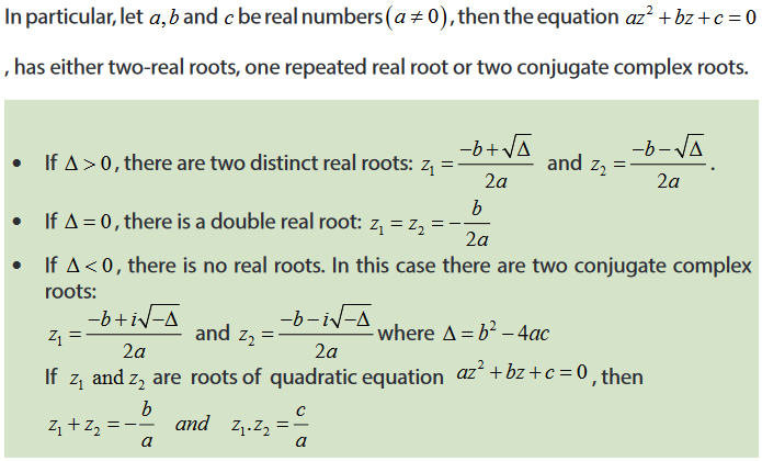
 1.1.6.2 Quadratic equations
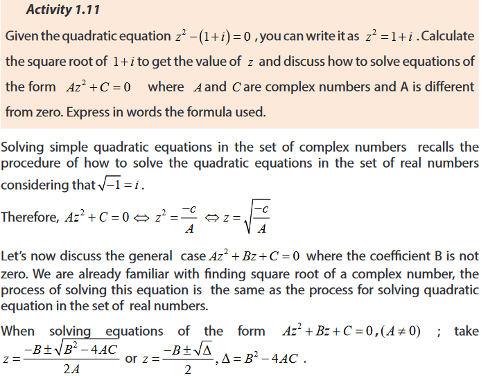


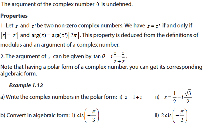
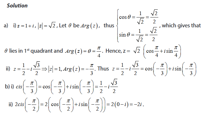
 1. 2 Polar form of a complex number1.2.1 Definition and properties of a complex number in polar form

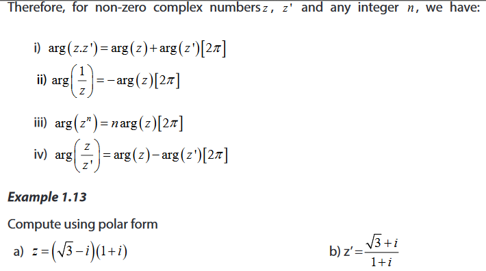
 1.2.2 Multiplication and division of complex numbers in polar form
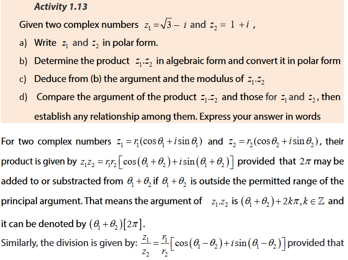


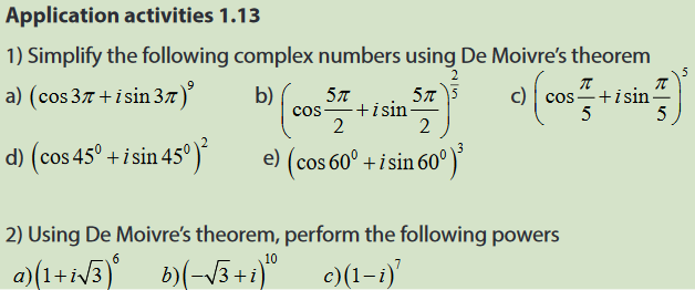
 1.2.3 Powers in polar form
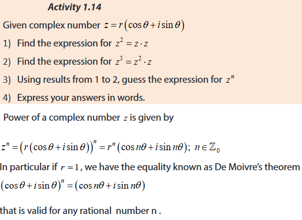


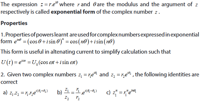
 1.3 Exponential form of complex numbers1.3.1 Definition of exponential form of a complex number
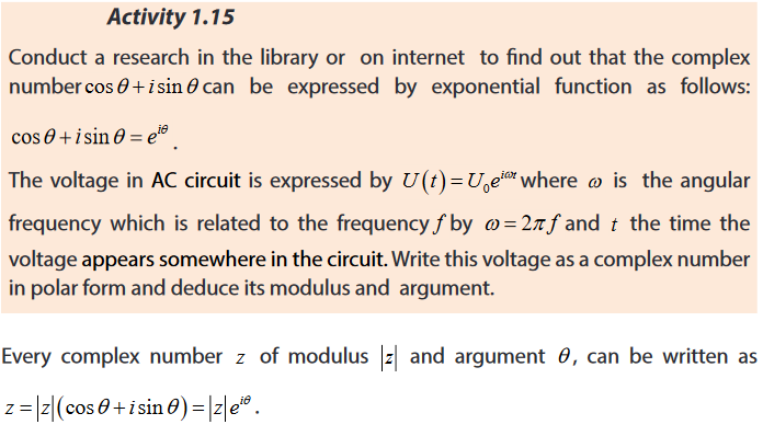
 In electrical engineering, the treatment of resistors, capacitors and inductors can be unified by introducing imaginary, frequency-dependent resistances for capacitor, inductors and combining all three (resistors, capacitors, and inductors) in a single complex number called the impedance. This approach is called phasor calculus. As we have seen, the imaginary unit is denoted by j to avoid confusion with i which is generally in use to denote electric current. Since the voltage in an ACcircuit is oscillating, it can be represented as
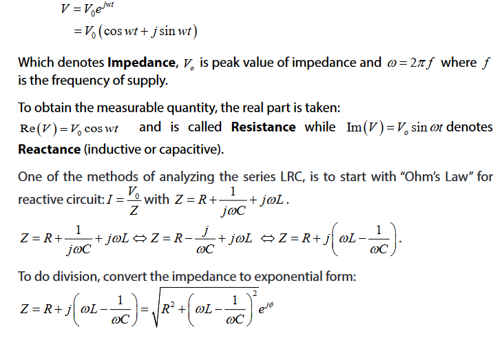


 1.3.2 Euler’s formulae
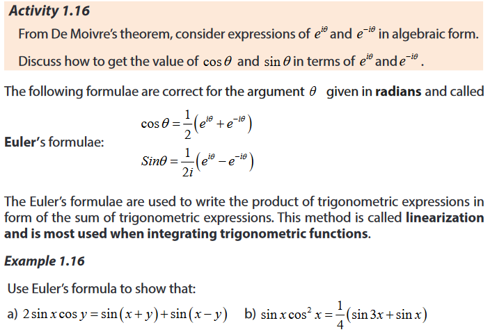

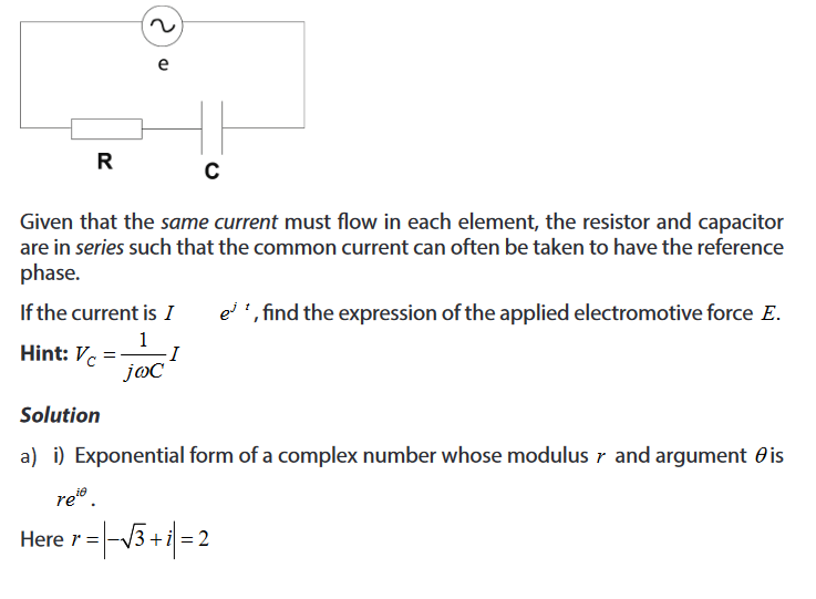
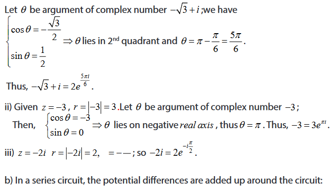
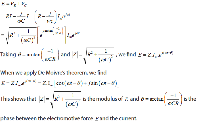
 1.3.3 Application of complex numbers in Physics

 End unit assessment

 Files: 2
UNIT2: LOGARITHMIC AND EXPONENTIAL FUNCTIONS
Key unit competence
Extend the concepts of functions to investigate fully logarithmic and exponential functions and use them to model and solve problems about interest rates, population growth or decay, magnitude of earthquake, etc.
Introductory activity

From the discussion, the function
Ft found in c) and the function ( )YF found in d) are respectively exponential function and logarithmic functions that are needed to be developed to be used without problems. In this unit, we are going to study the behaviour and properties of such essential functions and their application in real life situation.
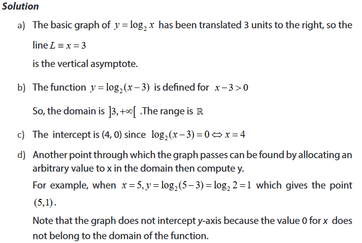
2. 1 Logarithmic functions
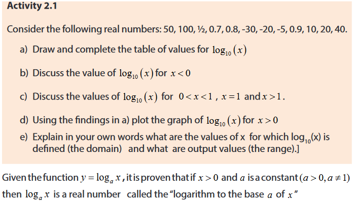
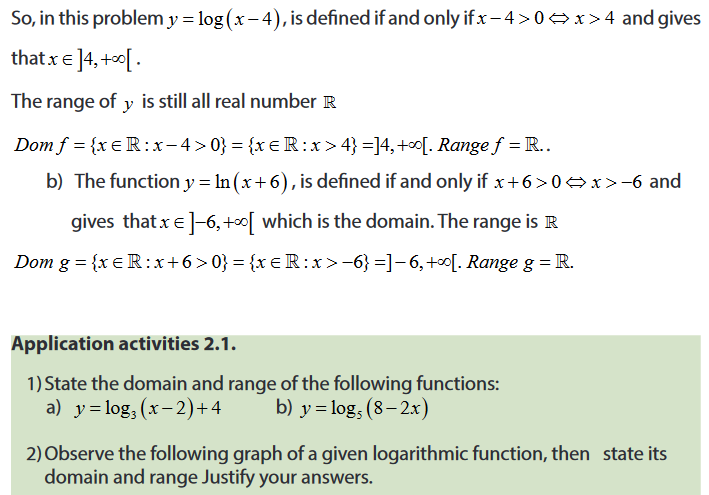
2.1.1 Domain of definition for logarithmic function


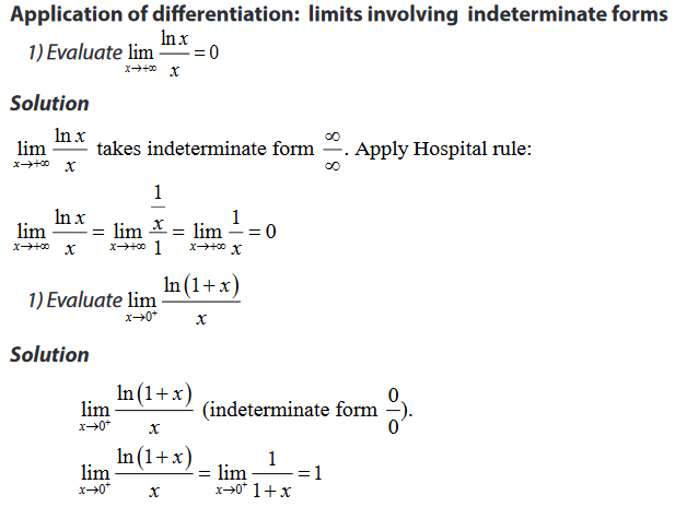
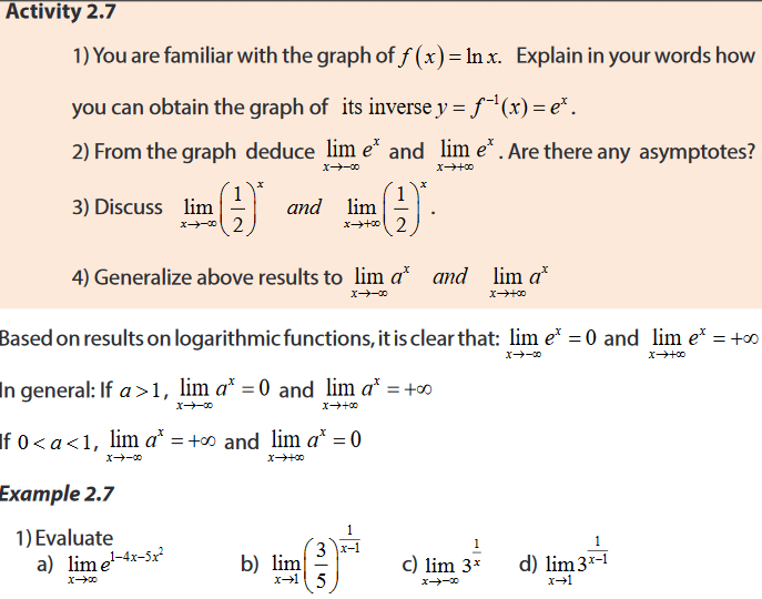
2.1.2 Limits and asymptotes of logarithmic functions


2.1.3 Continuity and asymptote of logarithmic functions


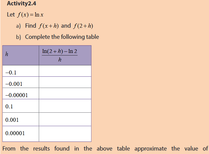
2.1.4. Differentiation of logarithmic functions


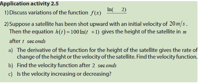
2.1.5 Variation of logarithmic function


Thus, 1110 1 1xxx−=⇔ =⇒=. If 1,x=
2. 2 Exponential functions
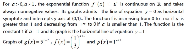
2.2.1 Domain of definition of exponential function


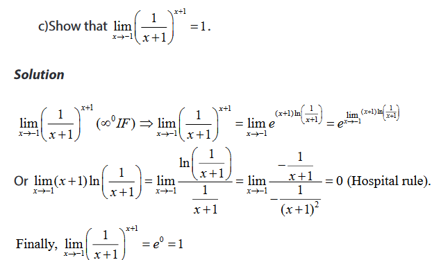
2.2.2 Limits of exponential functions


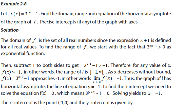
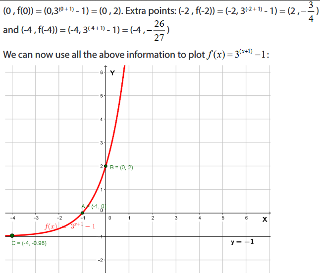
2.2.3. Continuity and asymptotes of exponential function


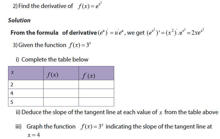
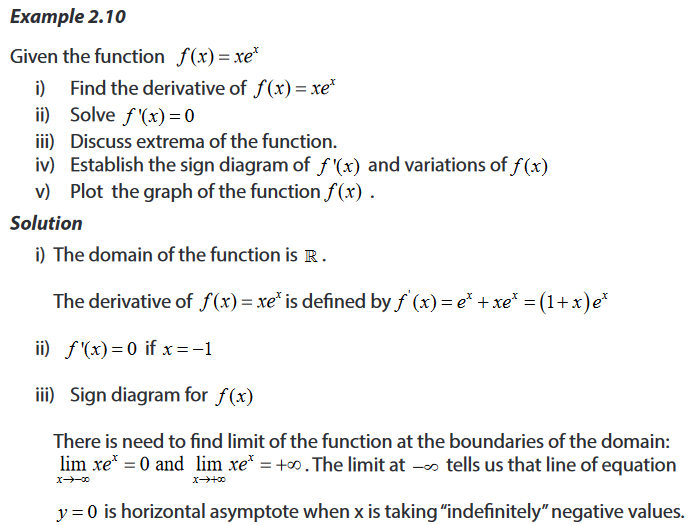
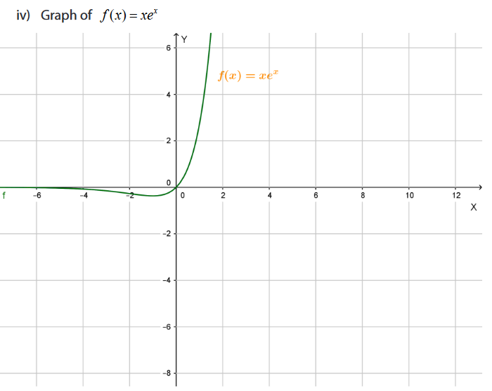
2.2.4. Differentiation of exponential functions


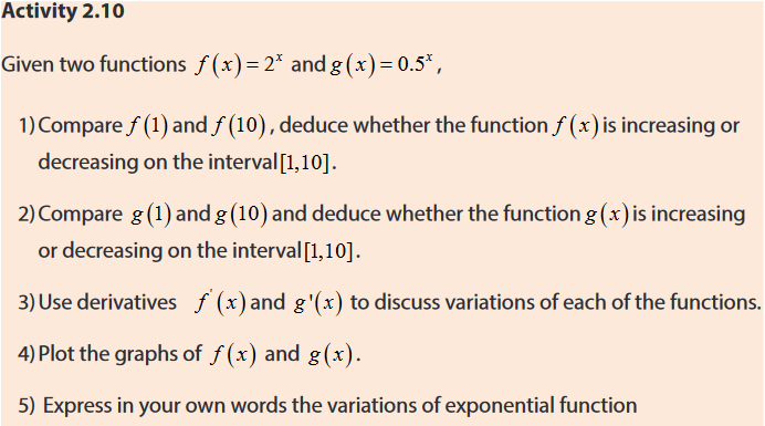
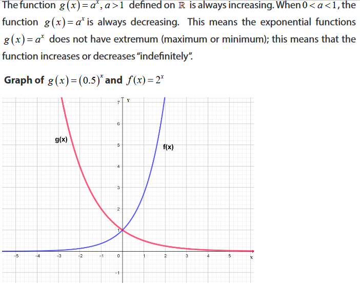
2.2.5 Variations of exponential functions


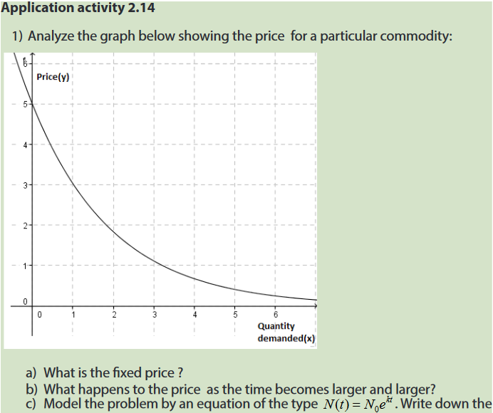
2. 3 Applications of logarithmic and exponential functions
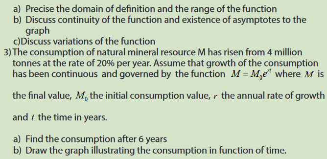
Logarithmic and exponential functions are very essential in pure sciences, social sciences and real life situations. They are used by bank officers to deal with interests on loans they provide to clients. Economists and demographists use such functions to estimate the number of population after a certain period and many researchers use them to model certain natural phenomena. We are going to develop some of these applications.
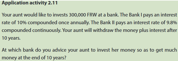
2.3.1 Interest rate problems
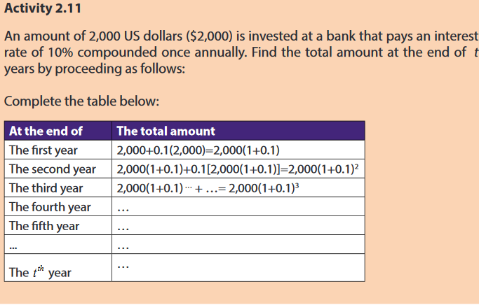
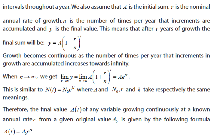
If a principal P is invested at an interest rate r for a period of t years, then the amount A (how much you make) of the investment can be calculated by the following generalised formula of the interest rate problems:


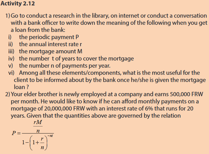
2.3.2 Mortgage problems


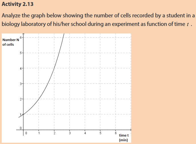
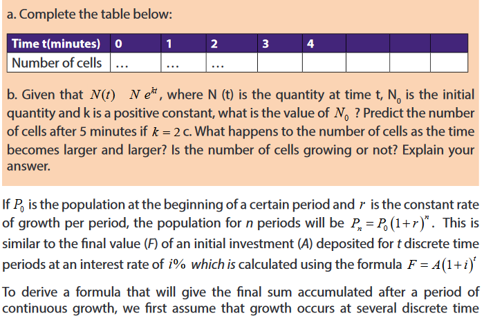
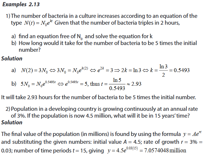
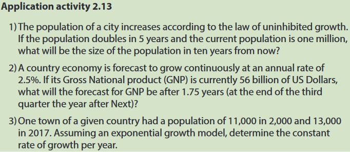
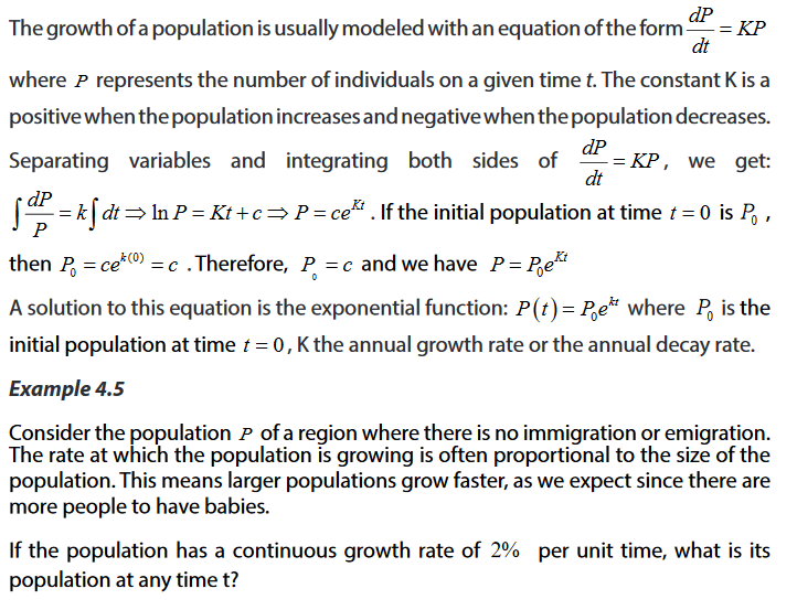
2.3.3 Population growth problems
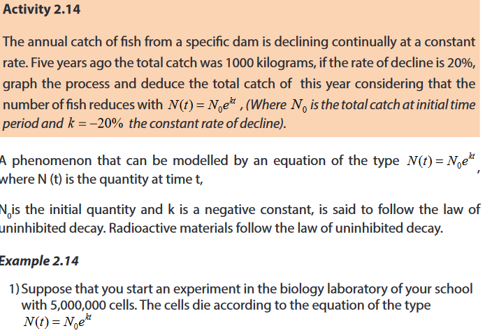
2.3.4 Uninhibited decay and radioactive decay problems


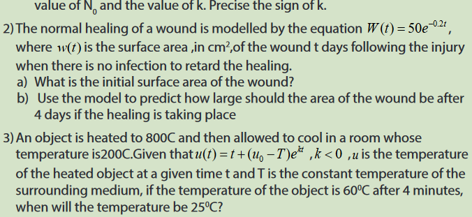
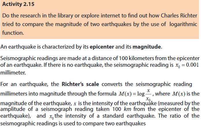
2.3.5 Earthquake problems


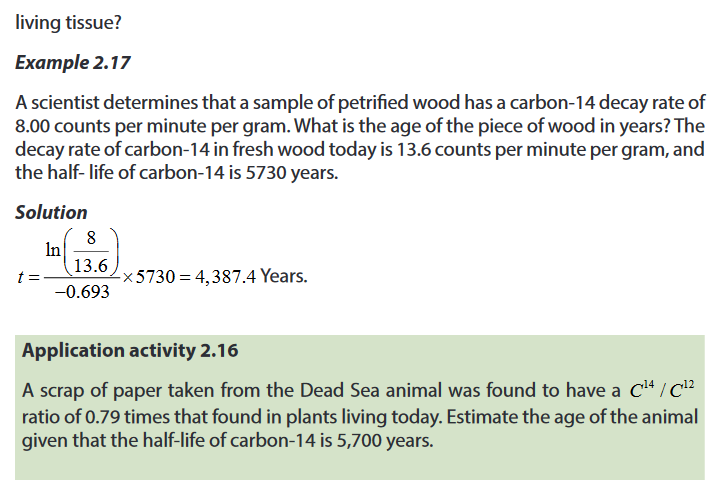
2.3.6 Carbon dating problems


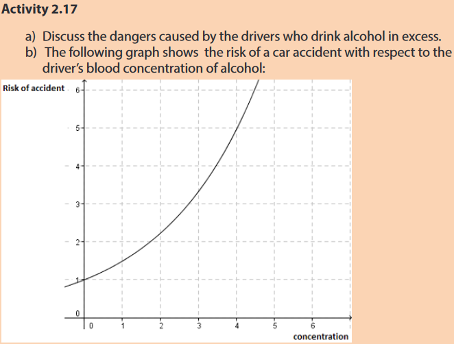
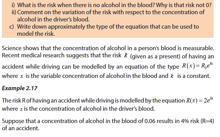
2.3.7 Problems about alcohol and risk of car accident


END UNIT ASSESSMENT

Unit 3: INTEGRATION
Key unit competence
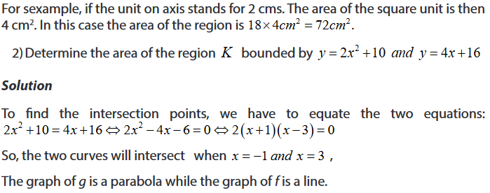
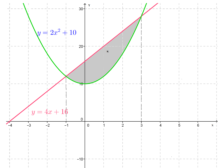
Use integration as an inverse of differentiation and then apply definite integrals to find area of plane shapes.
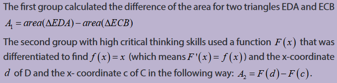
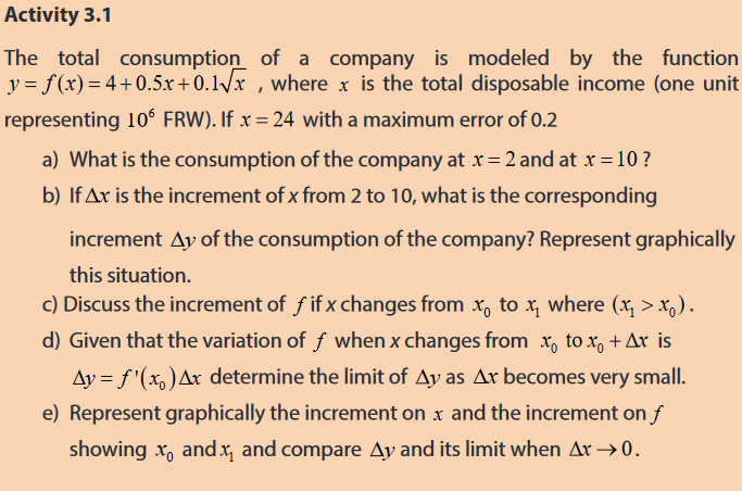
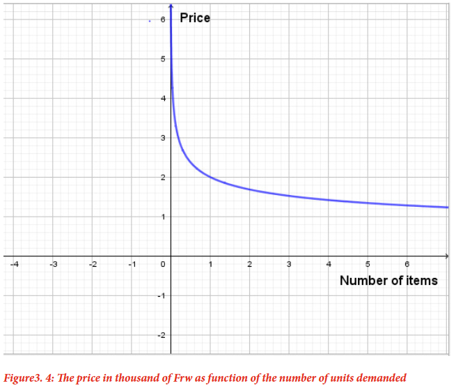
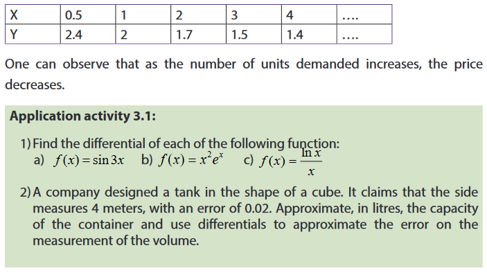
Introductory activity


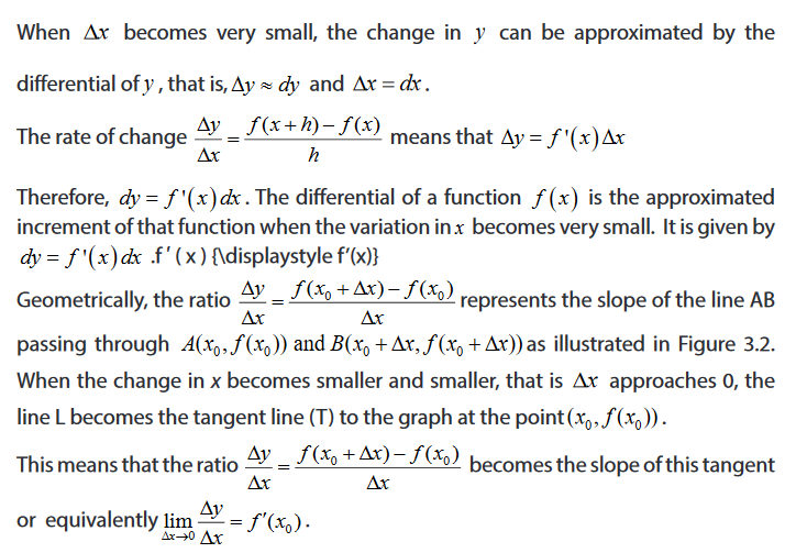
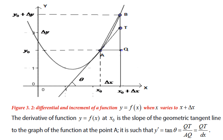
3. 1 Differential of a function


3.2 Anti-derivatives


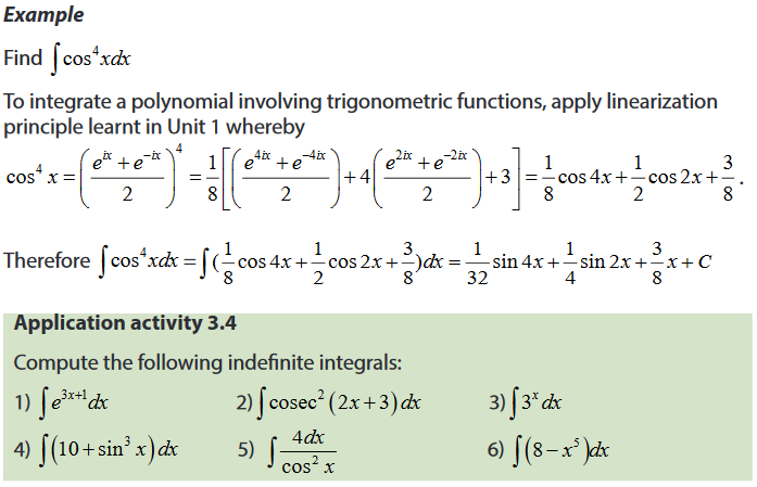
3.3 Indefinite integrals


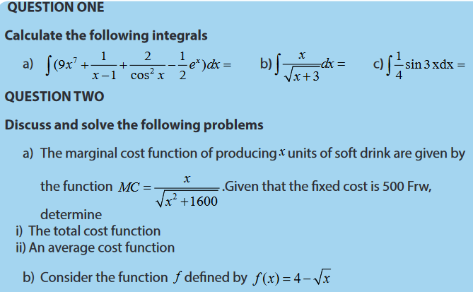
3.4. Techniques of integration
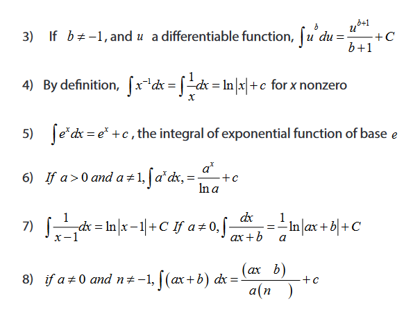
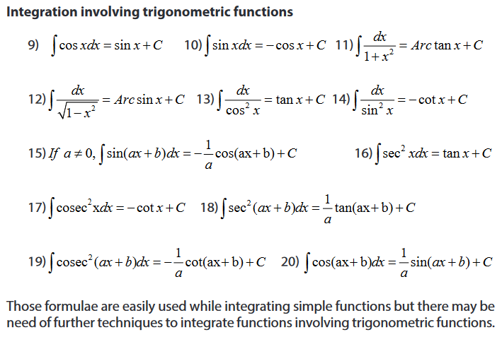
3.4.1 Basic integration formulae

3.4.2 Integration by changing variables


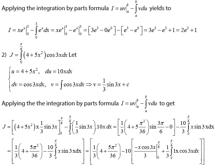
3.4.3 Integration by parts

When we integrate, we can find some functions which can’t be integrated immediately by using integration by changing variable method. To overcome that problem, you should use integration by parts or partial integration technique. In this, you have to find the integral of a product of two functions in terms of the integral of their derivative and anti-derivative.


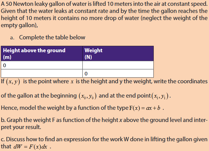
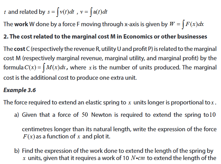
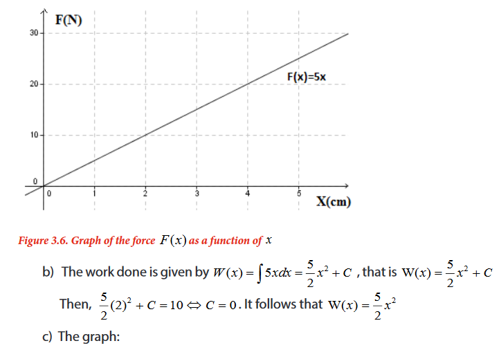
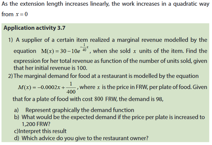
3.5 Applications of indefinite integrals


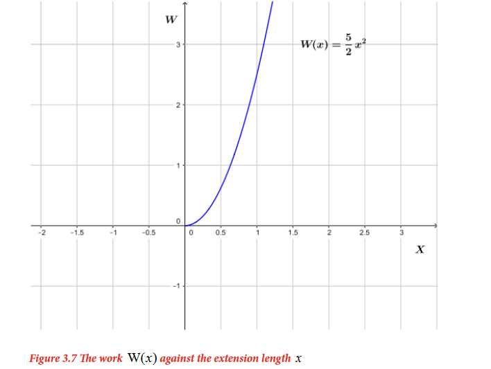
3.6 Definite integrals
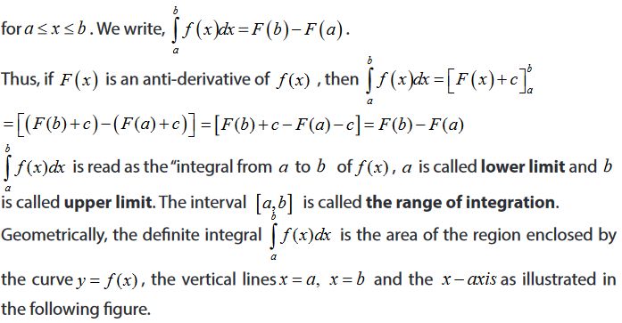
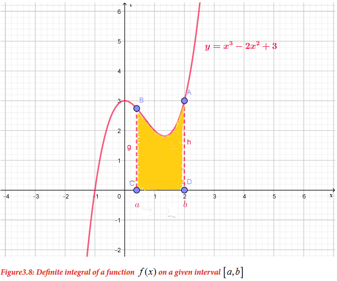
3. 6.1 Definition and properties of definite integrals


3.6.2 Techniques of Integration of definite integrals


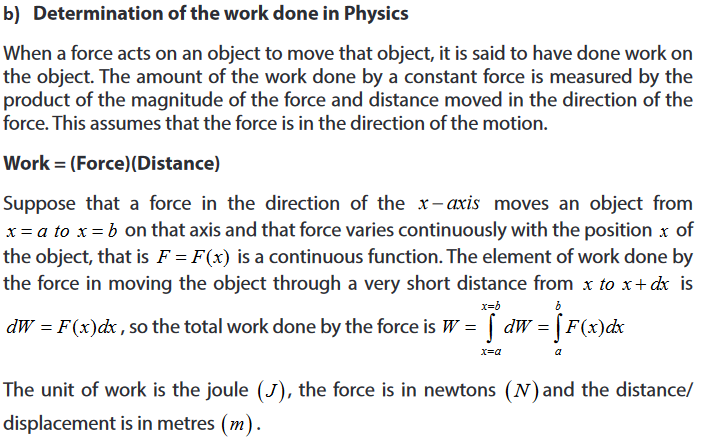
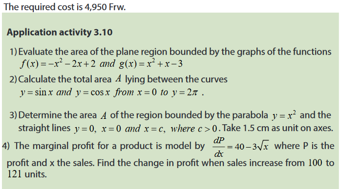
3.6.3 Applications of definite integrals


End unit assessment

Unit 4. ORDNINARY DIFFERENTIAL EQUATIONS
Key unit competence
Use ordinary differential equations of first and second order to model and solve related problems in Physics, Economics, Chemistry, Biology, Demography, etc.
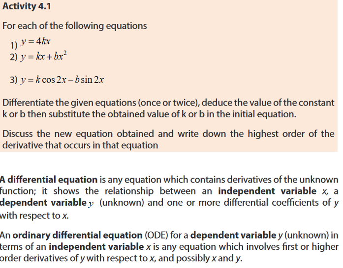
Introductory activity


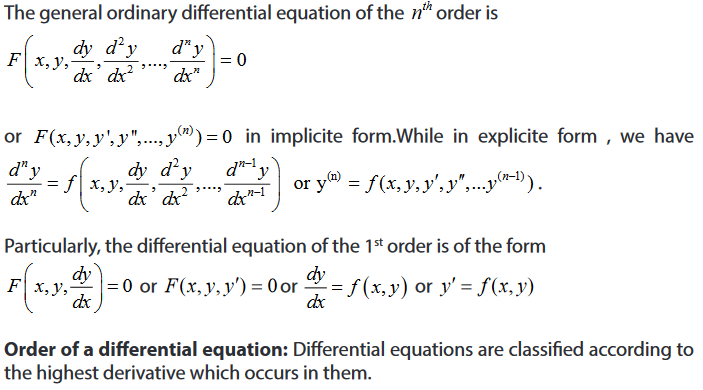
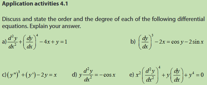
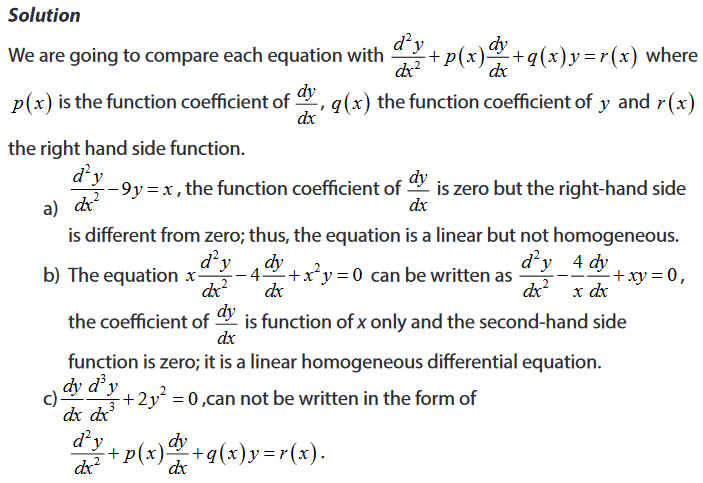
4.1 Definition and classification of differential equations

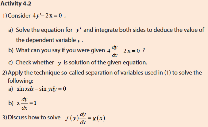
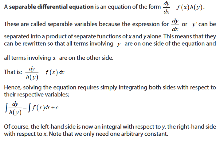
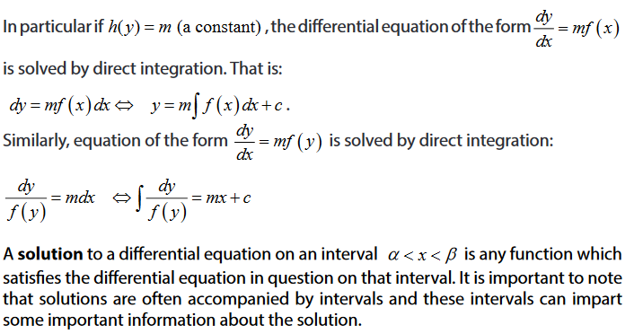
4.2 Differential equations of first order with separable variables


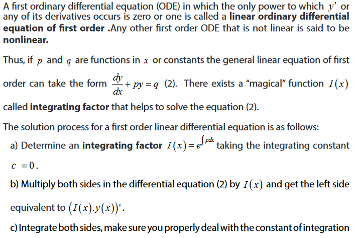
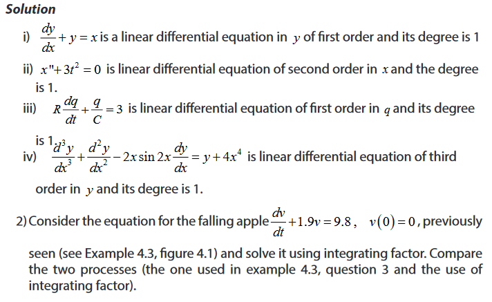
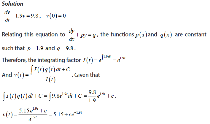
4.3. Linear differential equations of the first order


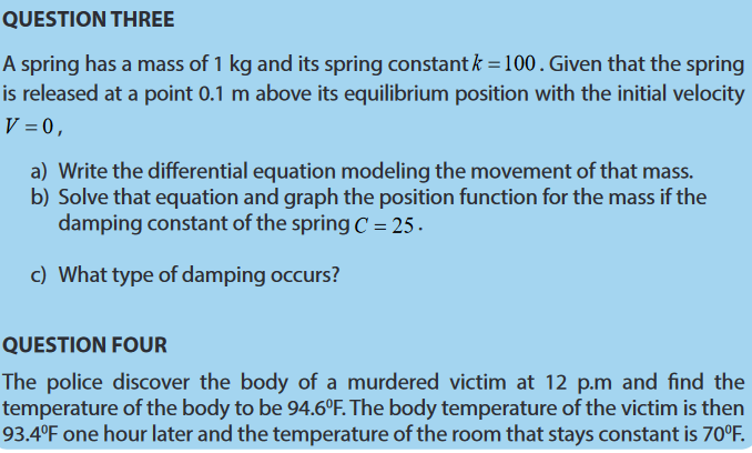
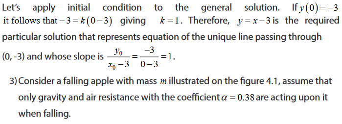
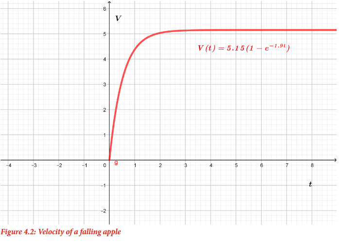
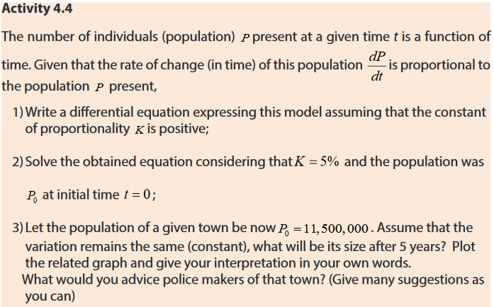
4.4 Applications of ordinary differential equations
4.4.1 Differential equations and the population growth


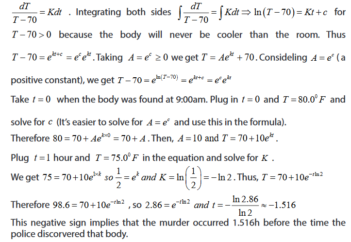
4.4.2 Differential equations and Crime investigation


4.4.3 Differential equations and the quantity of a drug in the body

exponentially.


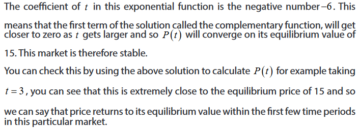
4.4.4 Differential equations in economics and finance


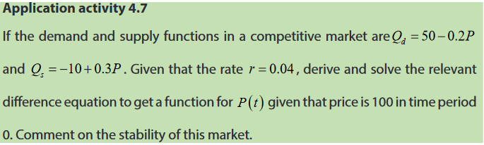
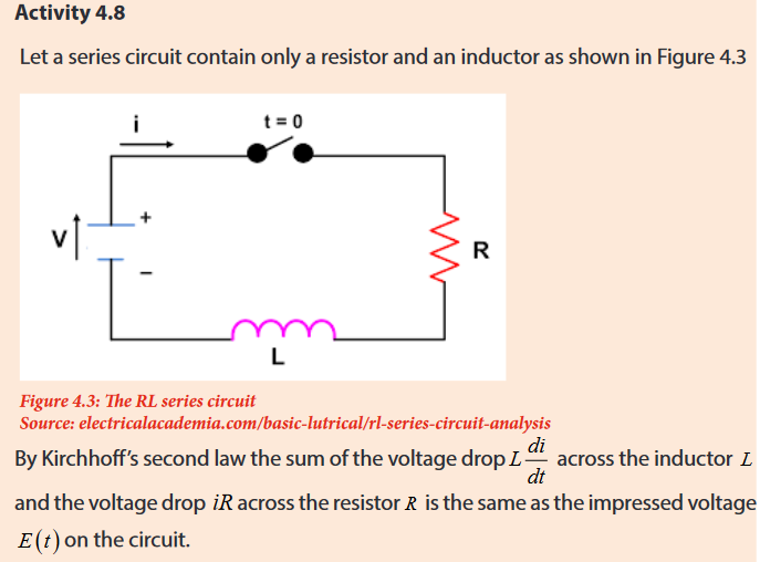
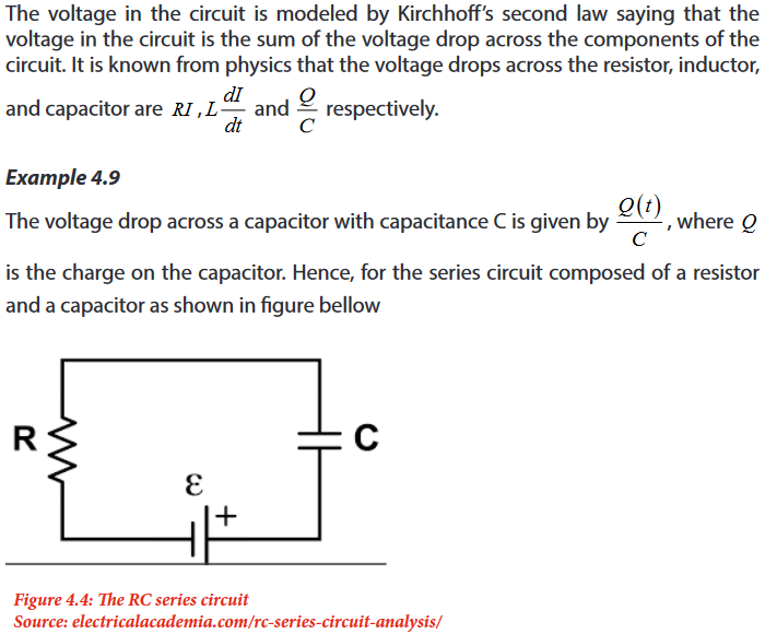
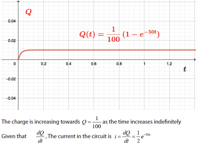
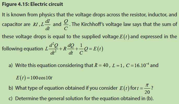
4.4.5 Differential equations in electricity (Series Circuits)


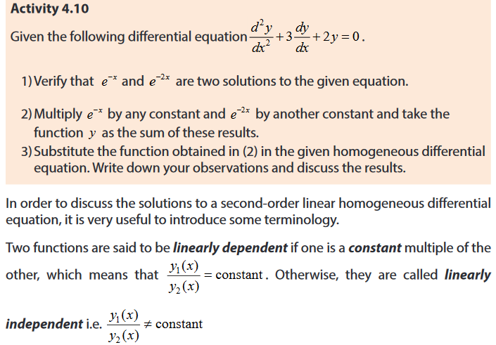
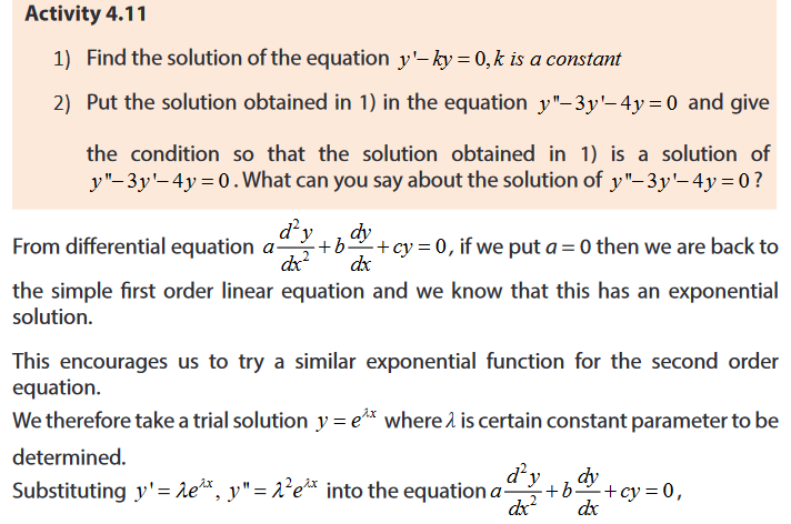
4.5. Introduction to second order linear homogeneous ordinary differential equations


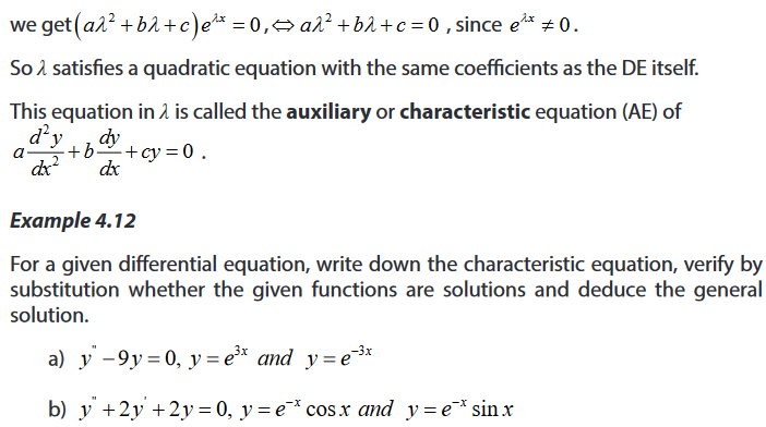
4.6 Solving linear homogeneous differential equations
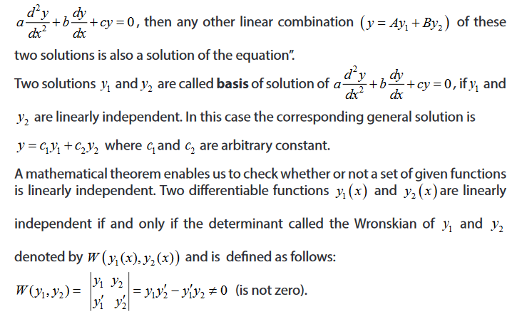
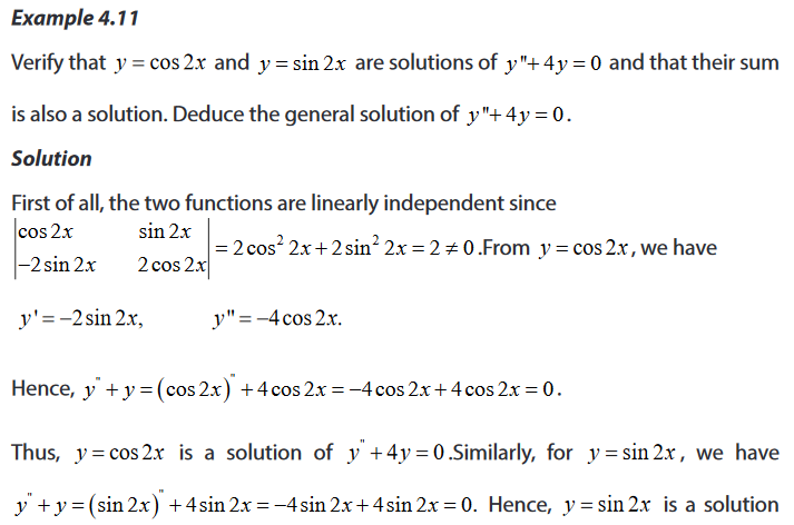
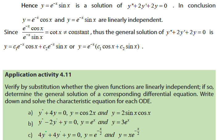
4.6.1. Linear independence and superposition principle


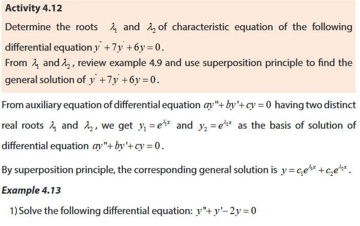
4.6.Characteristic equation of a second order differential equation


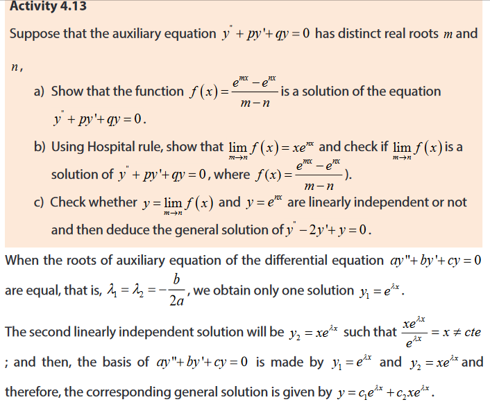
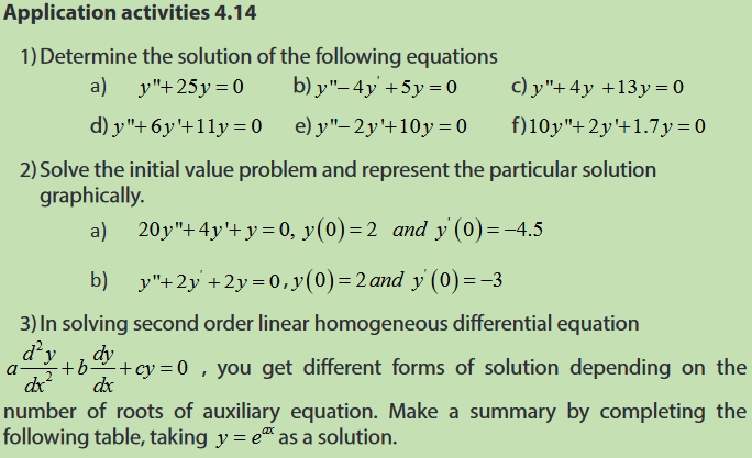
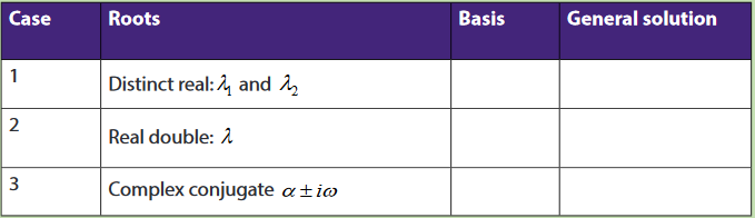
4.6.3. Solving DE whose Characteristic equation has two distinct real roots

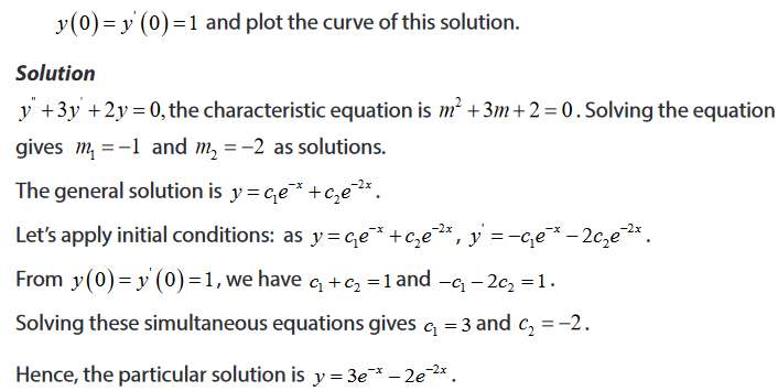


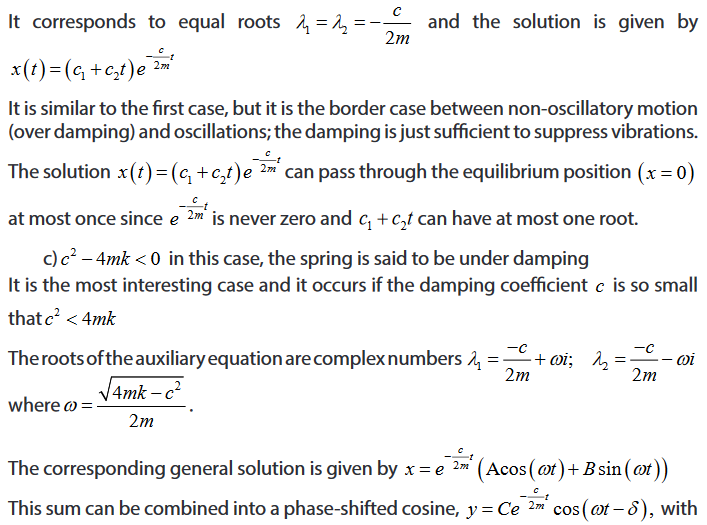
4.6.4. Solving DE whose Characteristic equation has a real double root repeated roots


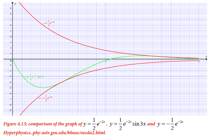
4.6.5. Solving DE whose characteristic equation has complex roots


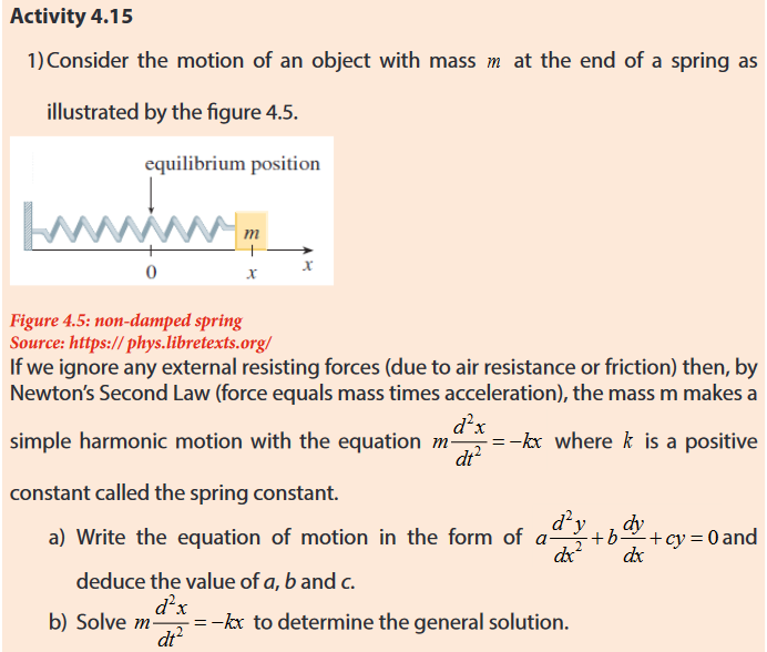
4.7. Applications of second order linear homogeneous differential equation


End unit assessment