Mathematics

Key unit competence 

Use the gradient of a straight line as a measure of rate of change and apply this to line tangents and normals to curves in various contexts. Use the concepts of differentiation to solve and interpret related rates and optimization problems in various contexts. 

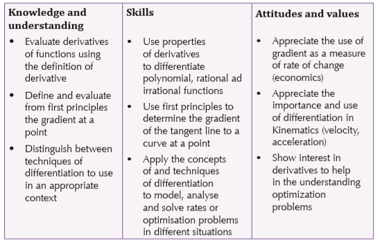
Learning objectives 

9.1 Concepts of derivative of a function

Definition

Mental task

You have learnt about gradients. What is the gradient of a line? How is it obtained?

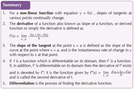
For a non-linear  function with equation y = f(x), slopes of tangents at various points continually change. 

The gradient of a curve at a point depends on the position of the point on the curve and is defined to be the gradient of the tangent to the curve at that point.

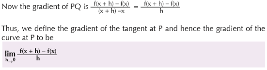
As Q approaches P along the curve, the gradient of the secant PQ approaches the gradient of the tangent at P. The gradient of the tangent at P is thus defined to be the limit of the gradient of the secant PQ as Q approaches P along the curve. i.e., as h → 0. 

Derivative of a function 

Activity 9.1 

In groups of five, carry out research to find out the meaning of the term derivative in mathematics. Present your findings to the rest of the class.

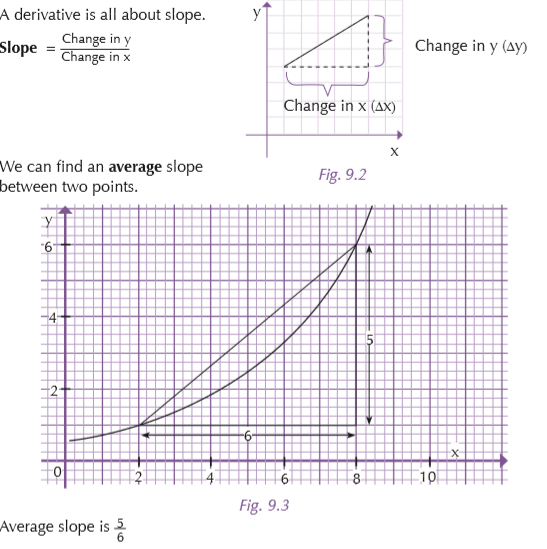
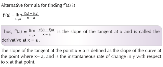
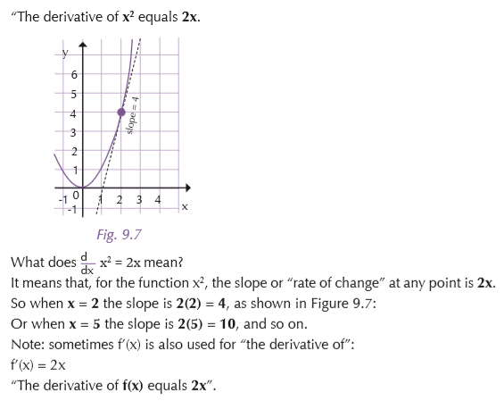
How do we get the slope (gradient) at a point? 

The derivative of a function y = f(x) at the point (x, f(x)) equals the slope of the tangent line to the graph at that point. 

Let us illustrate this concept graphically. 

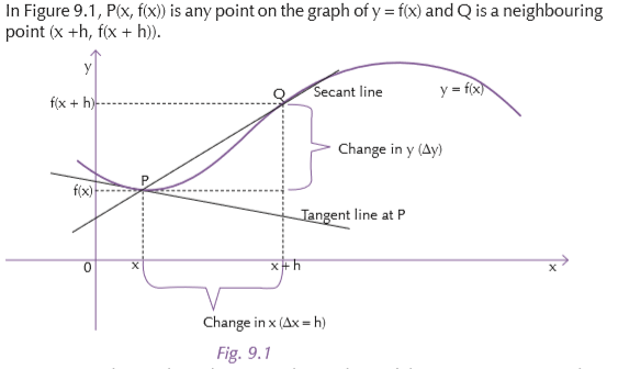
Let f be a real-valued function and P (x, f(x)) be a point on the graph of this function. Let there be another point Q in the neighbourhood of P.

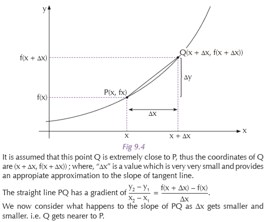
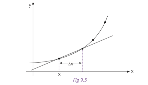
As the value of ∆x gets smaller, the two points get closer and the slope of PQ approaches that of the tangent line to the curve at P. As this happens the gradient of PQ will get closer to the slope of the tangent at P.

If we take this to the limit, as ∆x approaches 0, we will find the slope of the tangent at P and hence the gradient of the curve at P. 

Activity 9.2 

Work out the following in groups.

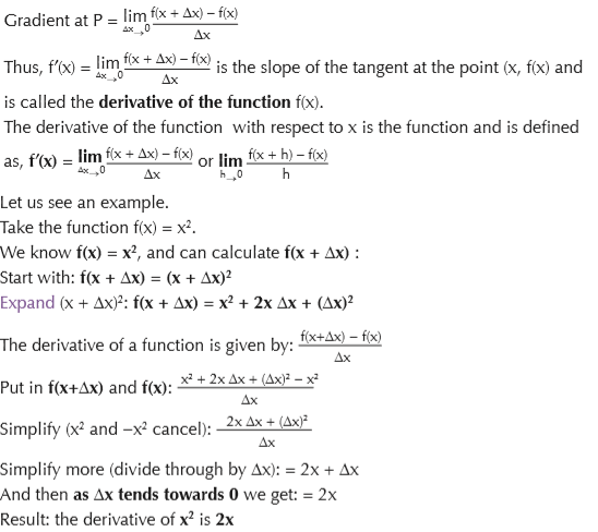
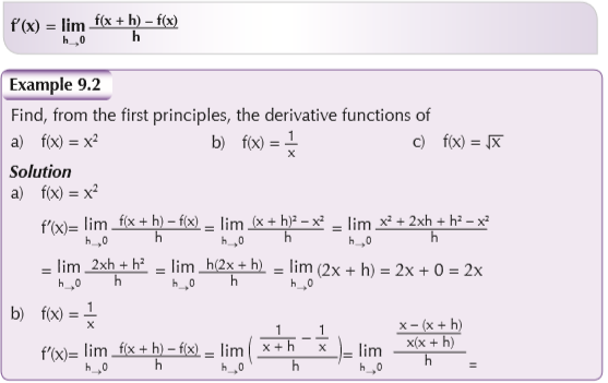
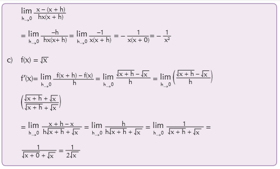
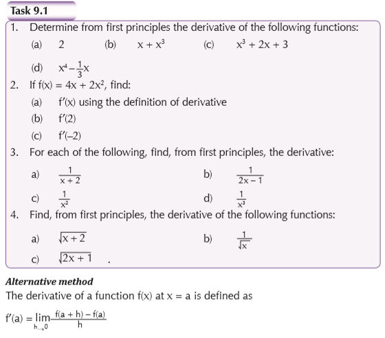
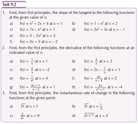
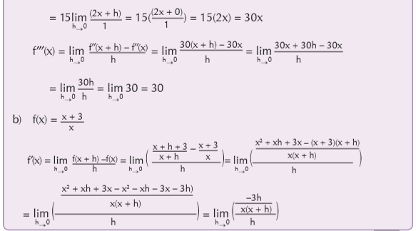
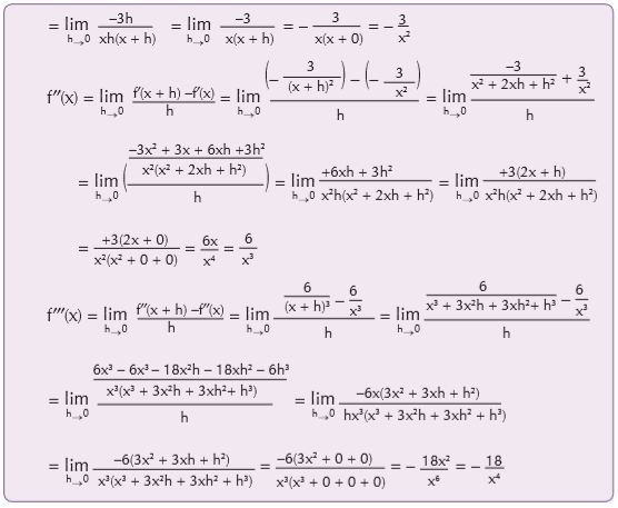
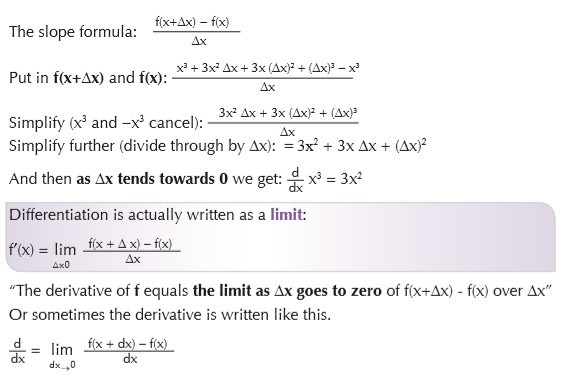
Differentiation from first principles 

Finding the slope using the limit method  is said to be using first principles, that is

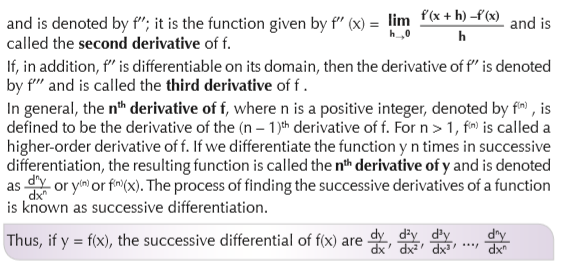
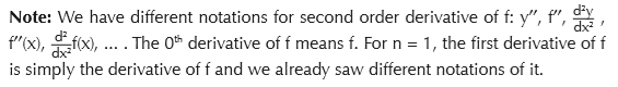
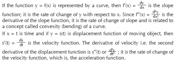
Higher order derivatives 

If f is a function which is differentiable on its domain, then f′ is a derivative function. If, in addition, f′ is differentiable on its domain, then the derivative of f′ exists 

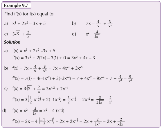
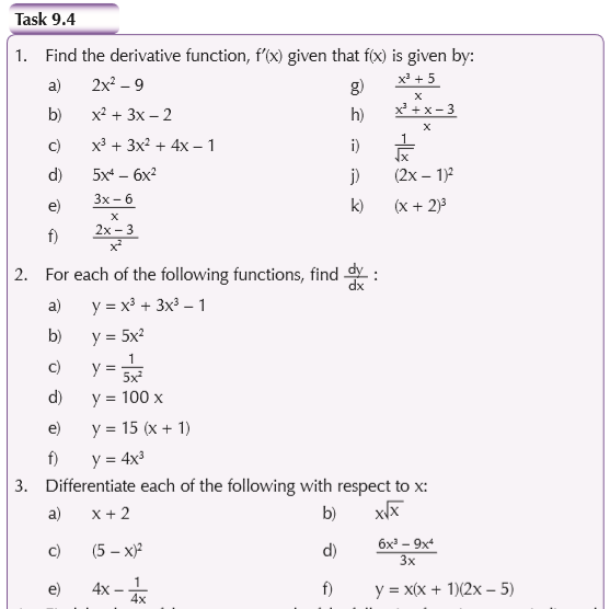
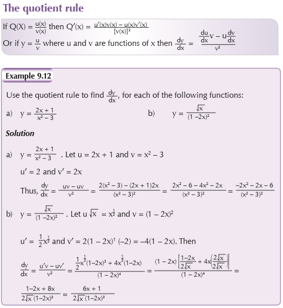
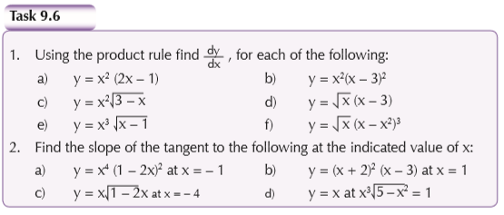
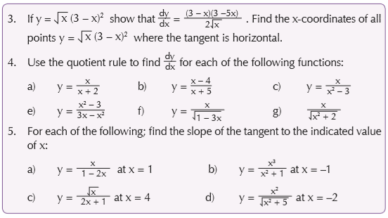
9.2 Rules of differentiation 

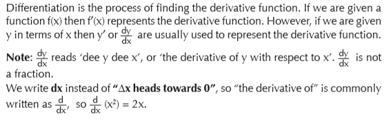
The process of finding a derivative is called “differentiation”.

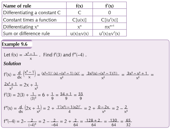
Below is the table containing basic rules which can be used to differentiate more complicated functions without using the differentiation from the first principles. 

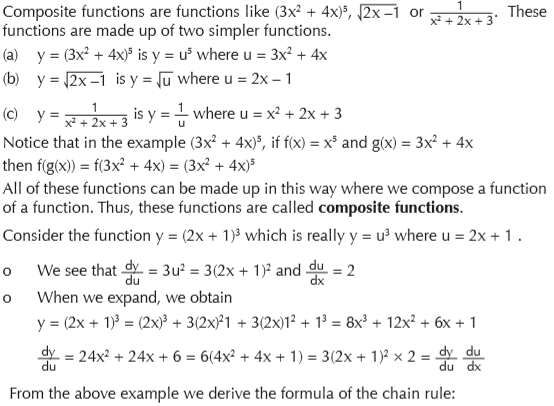
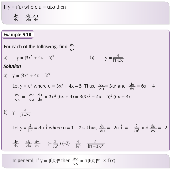
The chain rule 

9.3 Applications of differentiation

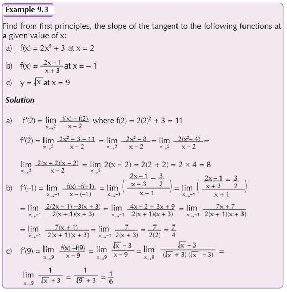
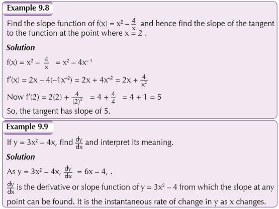
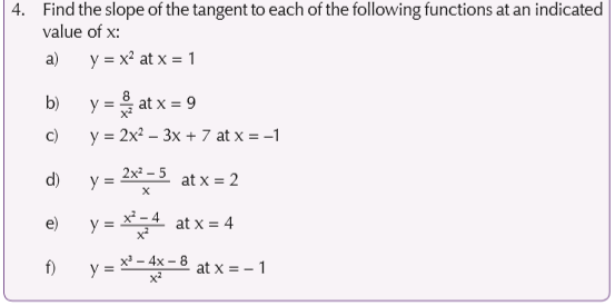
Geometric interpretation of derivatives 

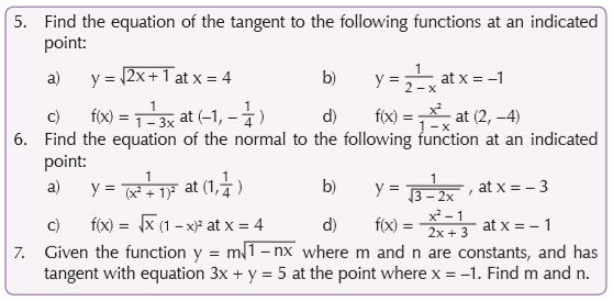
Equations of tangent and normal to a curve 

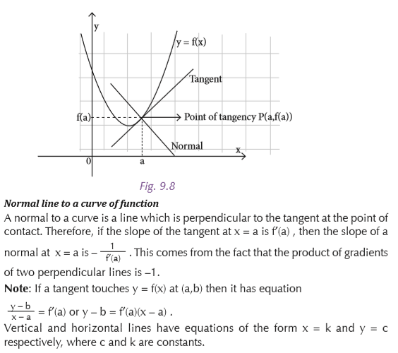
Tangent line to a curve of function 

Consider a curve y = f(x) . If P is the point with x-coordinate a, then the slope of the tangent at this point is f′(a) .The equation of the tangent is by equating slopes and is 

Mean value theorems 

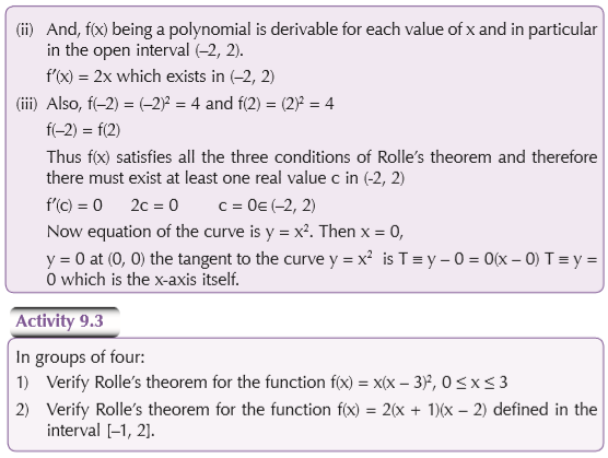
Rolle’s theorem

If f is continuous over a closed interval [a,b] and differentiable on the open interval (a,b), and if f(a) = f(b), then, there is at least one number c in ]a,b[ such that f′(c)=0.

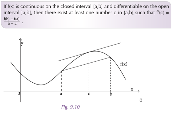
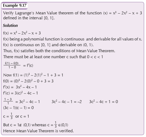
Lagrange’s mean value theorem

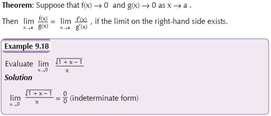
L’Hôpital theorem 

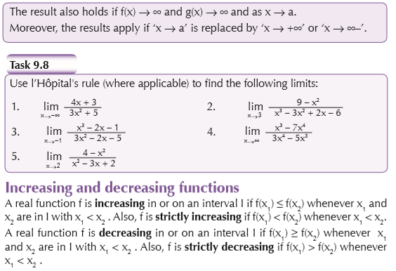
This is a rule for evaluating indeterminate forms. One of the forms of the rule is the following: 

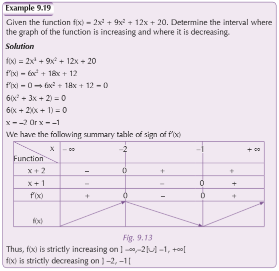
Meaning of the sign of the derivative 

If we recall that the derivative of a function yields the slope of the tangent to the curve of the function. It appears that a function is increasing at a point where the derivative is positive and decreasing where the derivative is negative.

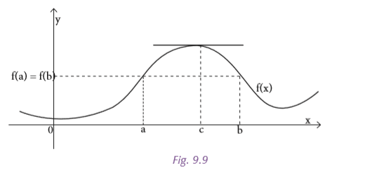
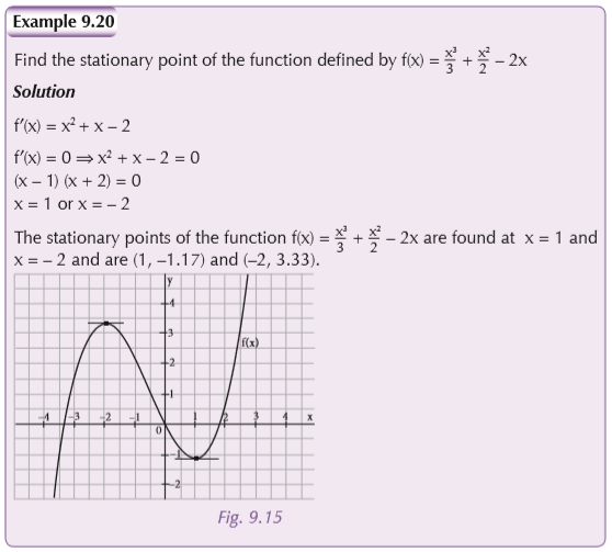
Stationary point 

This is a point on the graph y = f(x) at which f is differentiable and f′(x) = 0. The term is also used for the number c such that f′(c) . The corresponding value f(c) is a stationary value. A stationary point c can be classified as one of the following, depending on the behaviour of f in the neighbourhood of c: 

(i) A local maximum, if f′(x) > 0 to the left of c and f′(x) < 0 to the right of c, 

(ii) A local minimum, if f′(x) < 0 to the left of c and f′(c) > 0to the right of c, 

(iii) Neither local maximum nor minimum.

Note: Maximum and minimum values are termed as extreme values. 

The points a, b and c are stationary points.

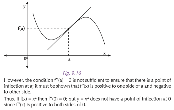
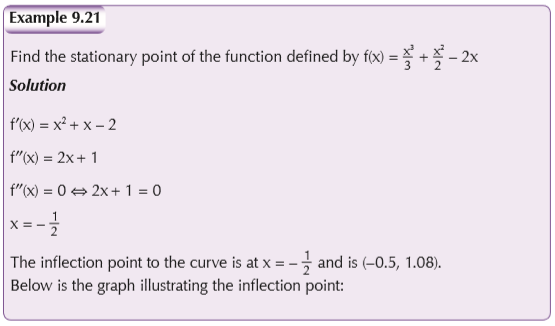
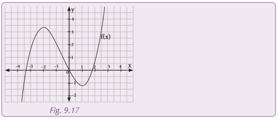
Point of inflection 

A point of inflection is a point on a graph y = f(x) at which the concavity changes. If f′ is continuous at a, then for y = f(x) to have a point of inflection at a it is necessary that f′′(a) =0, and so this is the usual method of finding possible points of inflection.

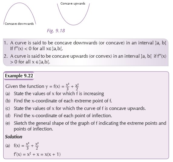
Concavity 

At a point of graph y = f(x), it may be possible to specify the concavity by describing the curve as either concave up or concave down at that point, as follows: 

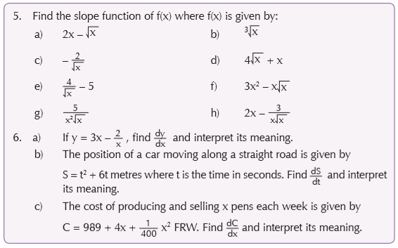
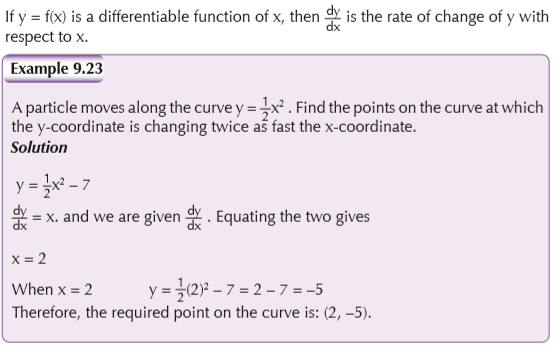
Rate of change problems

Mental task

We can use differentiation to help us solve many rate of change problems. Can you mention any such problems? 

Gradient as a measure of rate of change 

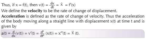
Kinematic meaning of derivatives 

Motion of a body on a straight line 

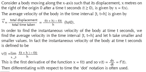
Velocity is a vector quantity and so the direction is critical. If the body is moving towards the right (the positive direction of the x-axis), its velocity is positive and if it is moving towards the left, its velocity is negative. Therefore, the body changes motion when velocity changes sign. A sign diagram of the velocity provides a deal with information regarding the motion of the body.

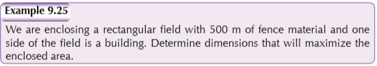
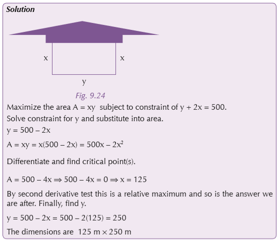
Optimization problems

Activity 9.4 

Carry out research on the meaning of optimization. Where is optimization applied?

Mathematical optimization is the selection of a best element (with regard to some criteria) from some set of available alternatives. 

In the simplest case, an optimization problem consists of maximizing or minimizing a real function by systematically choosing input values from within an allowed set and computing the value of the function.