Topic outline
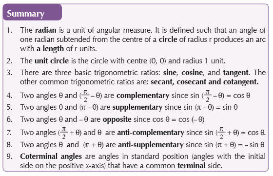
UNIT 1 : Fundamentals of trigonometry
Key unit competence
Use trigonometric circles and identities to determine trigonometric ratios and apply them to solve related problems.
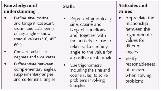
Learning objectives
1.1 Trigonometric concepts
The word trigonometry is derived from two Greek words: trigon, which means triangle, and metric, which means measure. So we can define trigonometry as measurement in triangles.
Angle and its measurements
Activity 1.1
In pairs, discuss what an angle is. Sketch different types of angles and name them: acute, obtuse, reflex, etc. Measure the angles to verify the sizes.
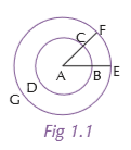
An angle is the opening that two straight lines form when they meet. In Figure 1.1, when the straight line FA meets the straight line EA, they form the angle we call angle FAE. We may also call it “the angle at the point A,” or simply “angle A.”
The two straight lines that form an angle are called its sides. And the size of the angle does not depend on the lengths of its sides.
Degree measure
To measure an angle in degrees, we imagine the circumference of a circle divided into 360 equal parts. We call each of those equal parts a “degree.” Its symbol is a small o: 1° = “1 degree.”
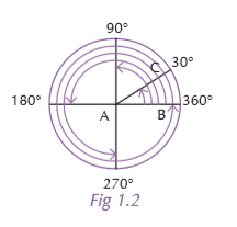
The measure of an angle, then, will be as many degrees as its sides include. To say that angle BAC is 30° means that its sides enclose 30 of those equal divisions. Arc BC is 30/180 of the entire circumference.
Radians
Activity 1.2
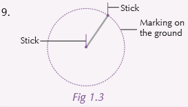
This activity will be carried out in the field. Each group will need: two pointed sticks, two ropes (each about 50 cm in length), black board protractor and metre rule.
1. Fix the pointed sticks, one at each end of the rope.
2. Place the sharp end of one of the sticks onto the ground.
3. With that point as the centre, let the tip of the 2nd stick draw a circle, radius 50 cm.
4. Take the 2nd rope also of length 50 cm and fit it on any part of the circumference (an arc).
5. Take the metre rule and draw a line from each of the ends of the rope to the centre of the circle.
6. Use the large protractor to measure the angle enclosed by the two lines. What do you get?
7. Compare your result with the rest of the groups. Are they almost similar?
8. Repeat the task using ropes of length 70 cm each. How do the results compare with the ones of 50 cm lengths?
The radian is a unit of angular measure. It is defined such that an angle of one radian subtended from the centre of a unit circle produces an arc with arc length of r.
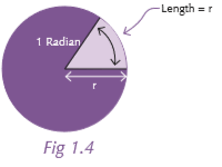
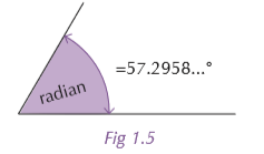
1 radian is about 57.2958 degrees. The radian is a pure measure based on the radius of the circle.
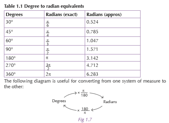
Degree-radian conversions
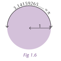
There are π radians in a half circle and 180° in the half circle.
So π radians = 180° and 1 radian
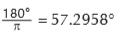 (approximately).
A full circle is therefore 2 radians. So there are 360°
per 2 radians, equal to
 or 57. 29577951°/ radian. Similarly, a right angle is
  radians and a straight angle is
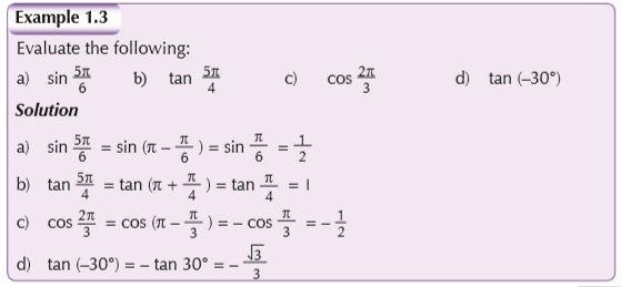
Example 1.1
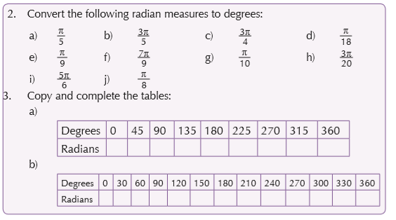
Convert 45° to radians in terms of π.
Solution

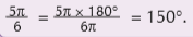
Example 1.2
Convert 5π/6 to degrees
Solution
The unit circle
Activity 1.3
Imagine a point on the edge of a wheel. As the wheel turns, how high is the point above the centre? In groups of four, represent this using a drawing.
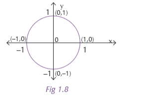
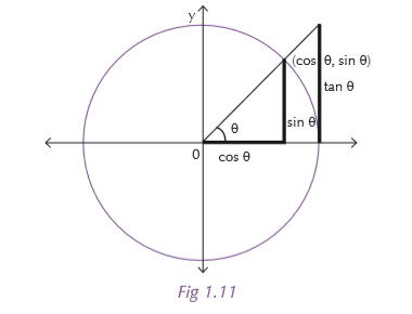
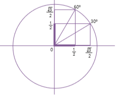
The unit circle is the circle with centre (0, 0) and radius 1 unit.
Definition of sine and cosine
Activity 1.4
Work in groups. Consider a point P(x,y) which lies on the unit circle in the first quadrant. OP makes an angle q with the x-axis as shown in Figure 1.9.
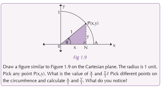
The x is the side adjacent to the angle q. And y is the side opposite the angle q.The radius of 1 unit is the hypotenuse.
Using right-angled triangle trigonometry:
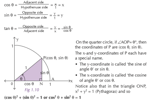
Note: We use cos2 q for (cos q)2 and sin2 q for (sin q)2.
Activity 1.5
In groups of three, use graph paper to draw a circle of radius 10 cm. Measure the half chord and the distance from the centre of the chord. Use various angles, say for multiples of 15°. Plot the graphs and determine the sines and the cosines.
We can also use the quarter unit circle to get another ratio. This is tangent which is written as 'tan' in short.
Trigonometric ratios
Activity 1.6
Carry out research on the trigonometric ratios. What are they? Define them.
There are three basic trigonometric ratios: sine, cosine, and tangent. The other common trigonometric ratios are: secant, cosecant and cotangent.
Trigonometric ratios in a right-angled triangle
In Figure 1.12, the side H opposite the right angle is called the hypotenuse. Relative to the angle q, the side O opposite the angle q is called the opposite side. The remaining side A is called the adjacent side.
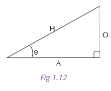
Trigonometric ratios provide relationships between the sides and angles of a right angle triangle. The three most commonly used ratios are sine, cosine and tangent.
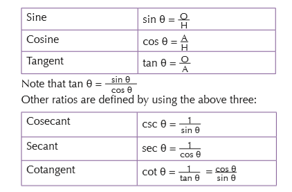
These six ratios define what are known as the trigonometric functions. They are independent of the unit used.
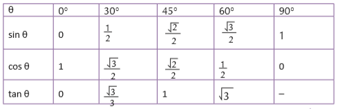
The trigonometric ratios of the angles 30º, 45º and 60º are often used in mechanics and other branches of mathematics. So it is useful to calculate them and know their values by heart.
The angle 45º
Activity 1.7
In pairs, draw an isosceles triangle where the two equal sides are 1 unit in length. Use Pythagoras' theorem to calculate the hypotenus.
In Figure 1.13, the triangle is isosceles. Hence the opposite side and adjacent sides are equal, say 1 unit.
The hypotenuse is therefore of length
 units (using Pythagoras’ theorem).
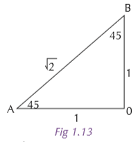

The angles 60º and 30º
Activity 1.8
In pairs, draw an equilateral triangle, ABC, of sides 2 units in length. Then draw a line AD from A perpendicular to BC. AD bisects BC giving BD = CD = 1.
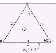
From this we can determine the following trigonometric ratios for the special angles 30º and 60º:

We can now complete the following table.
Complementary angles Two angles are complementary if their sum is

These two angles (30° and 60°) of Figure 1.15 are complementary angles, because they add up to 90°. Notice that together they make a right angle

Thus,
 are complementary angles.
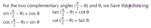
Supplementary angles
Two angles are supplementary if their sum is 180° (= π). The two angles (45° and 135°) of Figure 1.16 are supplementary angles because they add up to 180°.
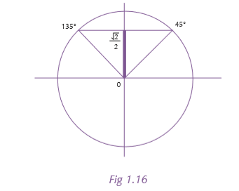
Notice that together they make a straight angle.

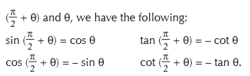
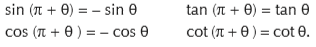
Thus, (π – q) and q are supplementary angles.
For the two supplementary angles (π – q) and q, we have the following:
sin (π – q) = sin q
cos (π – q) = – cos q
tan (π – q) = – tan q
cot (π – q) = – cot q.
Opposite angles
Two angles are opposite if their sum is 0. Thus, – q and q are opposite angles.
For the two opposite angles – q and q, we have the following:
sin (– q) = – sin q
cos (– q) = cos q
tan (– q) = – tan q
cot (– q) = – cot q.

Anti-complementary angles
Two angles are anti-complementary if their difference is

Notice that the two angles (60° and 150°) of Figure 1.18 are anti-complementary angles because their difference is 90°.

Thus,
 and q are anti-complementary angles.
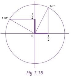
For the two anti-complementary angles
Anti-supplementary angles
Two angles are anti-supplementary if their difference is 180° (= π).
Notice that the two angles (30° and 210°) of Figure 1.19 are anti-supplementary angles, because their difference is 180°. Sin (210°)

Thus, (π + q) and q are anti-supplementary angles.
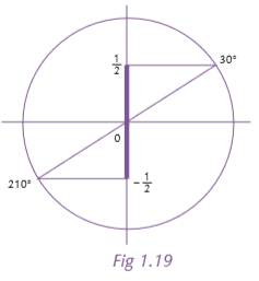
For the two anti-supplementary angles (π + q) and q, we have the following:
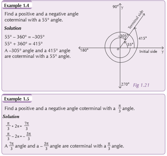
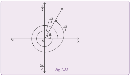
Coterminal angles
Coterminal angles are angles in standard position (angles with the initial side on the positive x-axis) that have a common terminal side. For example 30°, –330° and 390° are all coterminal.
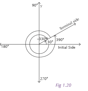
To find a positive and a negative coterminal angle with a given angle, you can add and subtract 360°, if the angle is measured in degrees, or 2π if the angle is measured in radians.

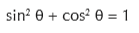
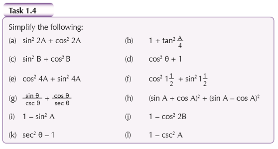
The trigonometric identities
In mathematics, an identity is an equation which is always true. There are many trigonometric identities, but the one you are most likely to see and use is,
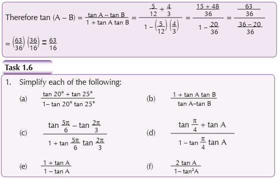
Addition formulae
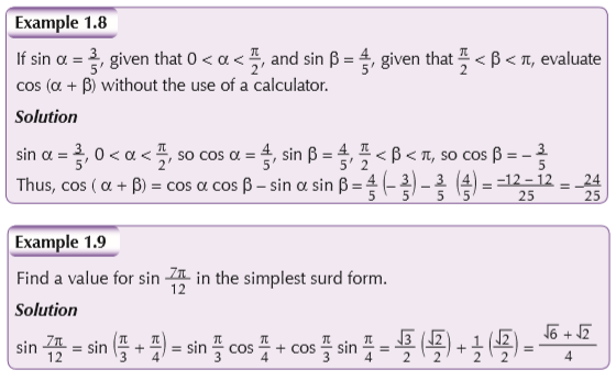
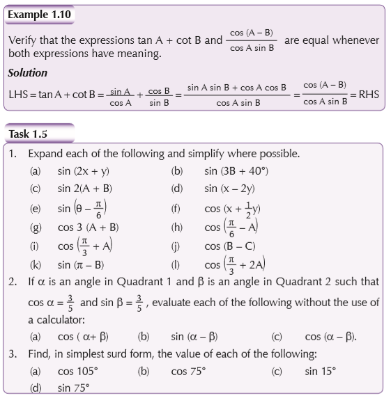
1. Cos (A – B) = cos A cos B + sin A sin B
2. Cos (A + B) = cos A cos B – sin A sin B
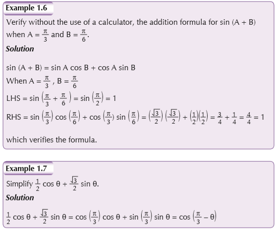
3. Sin (A + B) = sin A cos B + cos A sin B
4. Sin (A – B) = sin A cos B – cos A sin B
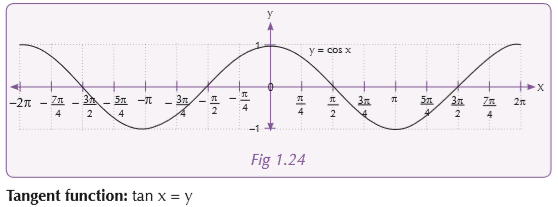
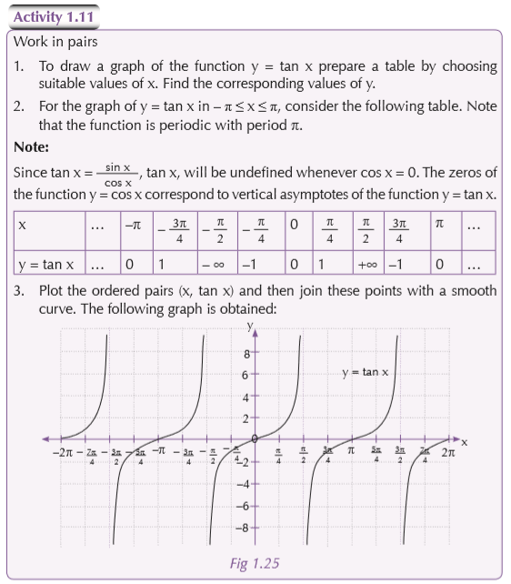
1.2 Reduction to functions of positive acute angles Graphs of some trigonometric functions
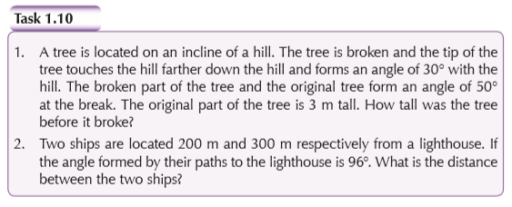
1.3 Triangles and applications
Triangles
The cosine rule
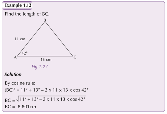
For any triangle with sides a, b, c and angles ABC as shown in Figure 1.26, the cosine rule is applicable:
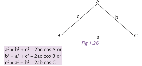
Note: For a right triangle at A i.e. A = 90°, cos A = 0. So a2 = b2 + c2 – 2bc cos A; reduces to a2 = b2 + c2 , and is the Pythagoras’Rule.
The cosine rule can be used to solve triangles if we are given:• two sides and an included angle
• three sides.
Rearrangement of the original cosine rule formulae can be used to find angles if we know all three sides. The formulae for finding angles are: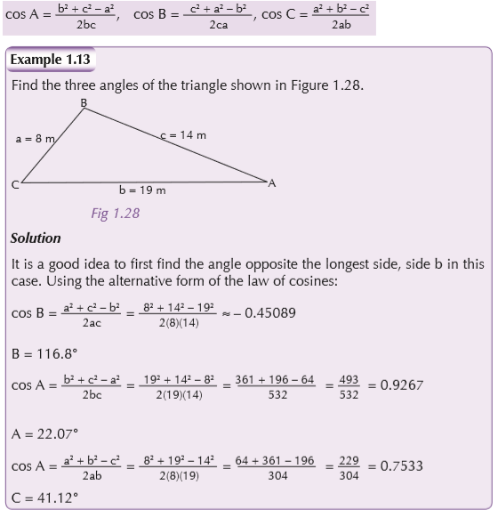

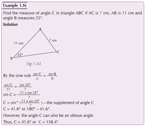
The sine rule
In any triangle ABC with sides a, b and c units in length, and opposite angles A, B and C respectively,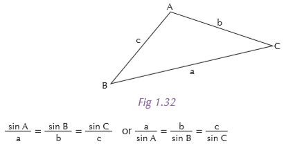
Note: The sine rule is used to resolve problems involving triangles given either:
• two angles and one side, or
• two sides and a non-included angle.

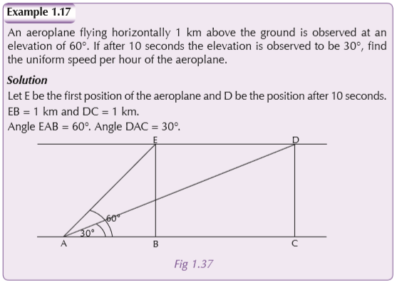
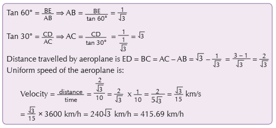
Air navigation
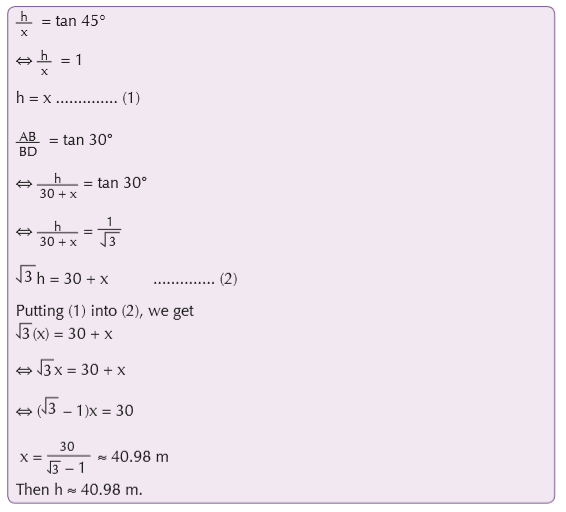
Inclined plane

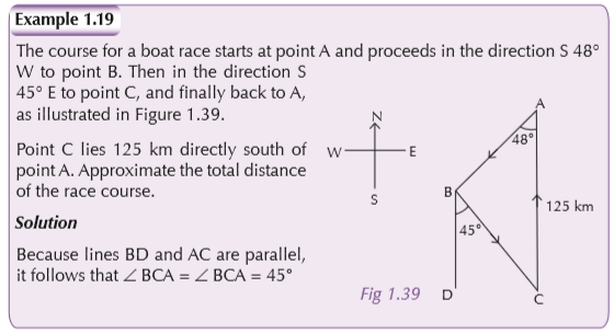
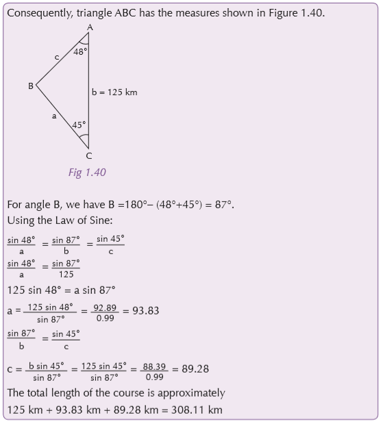
Bearing


UNIT 2 : Propositional and predicate logic
Key unit competence
Use mathematical logic to organise scientific knowledge and as a tool of reasoning in daily life.
Learning objectives
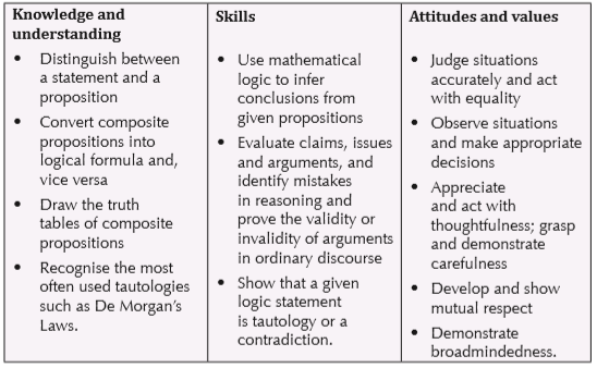
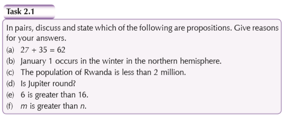
Activity 2.1
In groups of five, carry out research to distinguish between a statement and a proposition. Give examples of statements and propositions. Present your findings in class for discussion.
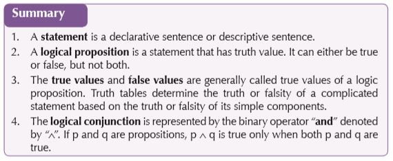
A statement is a declarative sentence or descriptive sentence. A logical proposition is a statement that has truth value. It can either be true or false, but not both.
In logic, we seek to express statements, and the connections between them in algebraic symbols. Logic propositions can be denoted by letters such as p, q, r, s, …
Below are some examples:
• r: 4 < 8
• s: If x = 4 then x + 3 = 7
• t: Nyanza is city in Rwanda
• p: What a beautiful evening!
The statements r, s and t are logic propositions. The statement p is not a logic proposition.
Recall that a proposition is a declarative sentence that is either true or false. Here are some more examples of propositions:
• All cows are brown.
• The Earth is farther from the sun than Venus.
• 2 + 2 = 5.
Here are some sentences that are not propositions.
1. "Do you want to go to the market?” Since a question is not a declarative sentence, it fails to be a proposition.
2. "Clean up your room.” Likewise, this is not a declarative sentence; hence, fails to be a proposition.
3. "2x = 2 + x.” This is a declarative sentence, but unless x is assigned a value or is otherwise prescribed, the sentence is neither true nor false, hence, not a proposition.
Each proposition can be assigned one of two truth values. We use T or 1 for true and use F or 0 for false.
2.2 Propositional logic
The simplest and most abstract logic we can study is called propositional logic.
Truth tables
The true values and false values are generally called true values of a logic proposition. At each proposition, corresponds an application that is a set {True, False} denoted by {T,F} or {1,0}.
You can use truth tables to determine the truth or falsity of a complicated statement based on the truth or falsity of its simple components.
A statement in sentential logic is built from simple statements using the logical connectives ∼, ∧, ∨, ⇒ and ⇔. We can construct tables which show how the truth or falsity of a statement built with these connectives depends on the truth or falsity of its components.
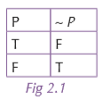
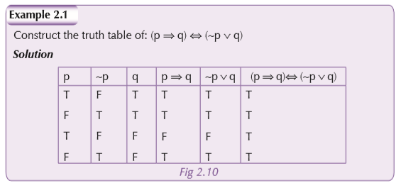
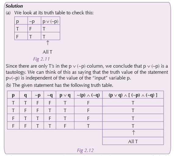
Figure 2.1 is the table for negation:
This table (Figure 2.1) is easy to understand. If p is true, its negation ∼ p is false. If p is false, then ∼ p is true}.
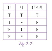
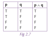
In Figure 2.2, p ∧ q should be true when both p and q are true, and false otherwise:
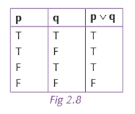
In Figure 2.3, p ∨ q is true if either p is true or q is true (or both). It is only false if both p and q are false.

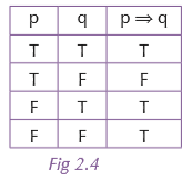
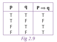
Figure 2.4 shows the table for logical implication:
There are 2n different possibilities of truth values given n logic propositions:
i. In the case of one proposition p there are 21 = 2 possibilities p : T or F
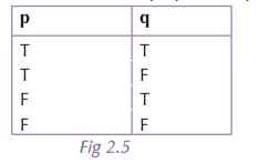
ii. In the case of two propositions p and q there are 22 = 4 possibilities
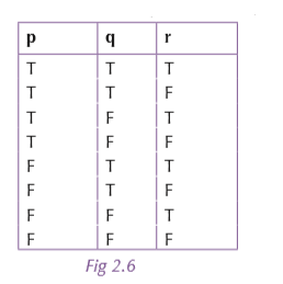
iii. The case of three propositions p, q and r there are 23 = 8 possibilities
Negation of a logic proposition (statement)
Activity 2.2
You are given a statement P:I go to school. What is the negative statement?
Logical negation is represented by the operator “NOT” denoted by "∼ or ¬ ”. The negation of the proposition p is the proposition ∼p which is true if p is false and false if p is true.
For example:
1. p : The lion is a wild animal; ∼p. The lion is not a wild animal.
2. q :3 < 7; ∼q: 3 ≥ 7
Logical connectives
Activity 2.3
You are given two statements:
p:I study Maths
q:I study English.
What do you say if you combine the two statements?
Propositions are combined by means of connectives such as and, or, if … then and if and only if and they are modified by not.
1. Conjunction
The logical conjunction is represented by the binary operator “and” denoted by "∧" . If p and q are propositions, p ∧ q is true only when both p and q are true. See Figure 2.7.
2. Disjunction
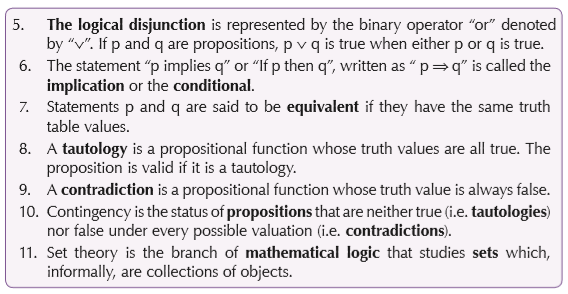
The logical disjunction is represented by the binary operator “or” denoted by “∨”. If p and q are propositions, p ∨ q is true when either p or q is true. See Figure 2.8
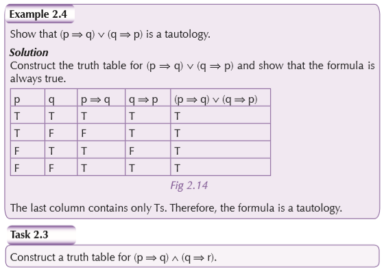
3. Implication
The statement “p implies q” or “if p then q”, written as “p ⇒ q” is called the implication or the conditional. In this setting, p is called “the premise, hypothesis or antecedent of the implication” and q is “the conclusion or the consequence of the implication”. p ⇒ q is false only when the antecedent p is true and the consequence q is false.
The statement p ⇒ q, when p is false, is sometimes called “a vacuous statement”. The converse of p ⇒ q is the implication q ⇒ p. If an implication is true, then its converse may or may not be true.
4. Equivalence
Statements p and q are said to be equivalent if they have the same truth table values. The corresponding logical symbols are "⇔" and “≡”, and sometimes “iff”.
The biconditional p ⇔ q read as “p is .... if and only if q” is true only when p and q have the same truth values

Note: The order of operations for the five logical connectives is as follows:
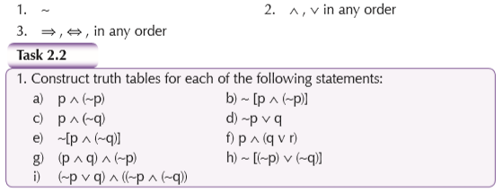
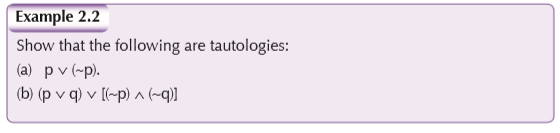
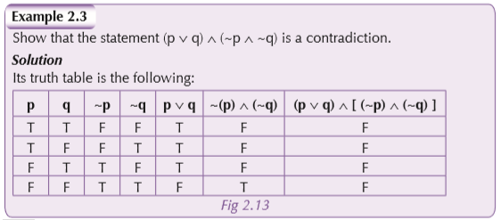
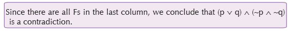
Tautologies and contradictions
A compound statement is a tautology if its truth value is always T, regardless of the truth values of its variables. It is a contradiction if its truth value is always F, regardless of the truth values of its variables. Notice that these are properties of a single statement, while logical equivalence always relates two statements.
When a statement is a tautology, we also say that the statement is tautological. In common usage this sometimes simply means that the statement is convincing. We are using it for something stronger: the statement is always true, under all circumstances. In contrast, a contradiction, or contradictory statement, is never true, under any circumstances.
Contingency
Contingency is the status of propositions that are neither true (i.e. tautologies) nor false under every possible valuation (i.e. contradictions).
Logically equivalent proposition
Two statements X and Y are logically equivalent if X ⇔ Y is a tautology. Another way to say this is: For each assignment of truth values to the simple statements which make up X and Y, the statements X and Y have identical truth values.
From a practical point of view, you can replace a statement in a proof by any logically equivalent statement.
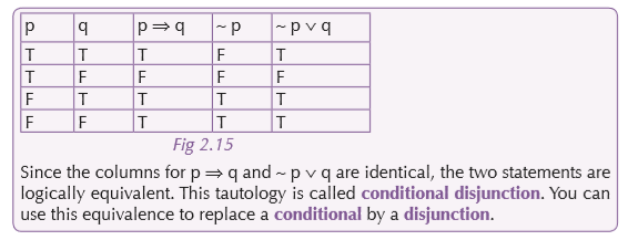
To test whether X and Y are logically equivalent, you could set up a truth table to test whether X ⇔ Y is a tautology; that is, whether X ⇔ Y ”has all Ts in its column”. However, it’s easier to set up a table containing X and Y and then check whether the columns for X and for Y are the same.
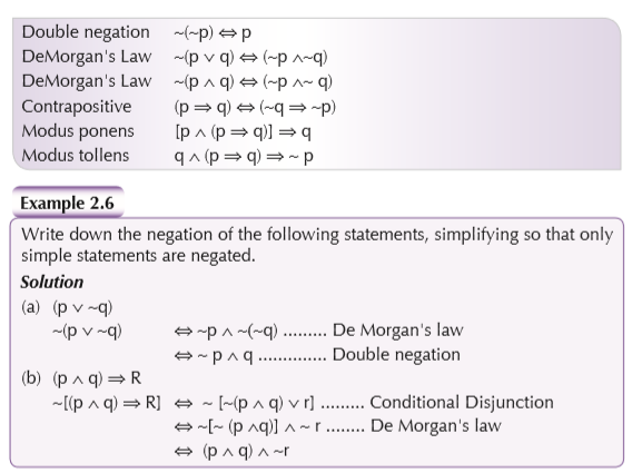
De Morgan’s Law For any two propositions p and q, the following hold:
1. ∼(p ∨ q)= ∼p ∧ ∼q
2. ∼(p ∧ q) = ∼p v ∼q
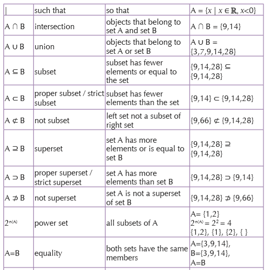
Given two sets A, B in the universal set U:
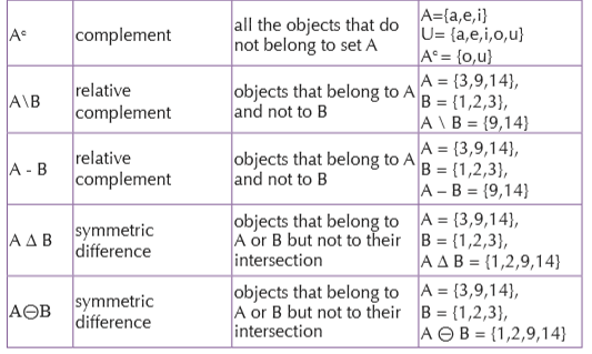
(A ∪ B)′ = A′ ∩ B′
(A ∩ B)′ = A′ U B′
There are an infinite number of tautologies and logical equivalences. A few examples are given below.
2.3 Predicate logic
Propositional functions
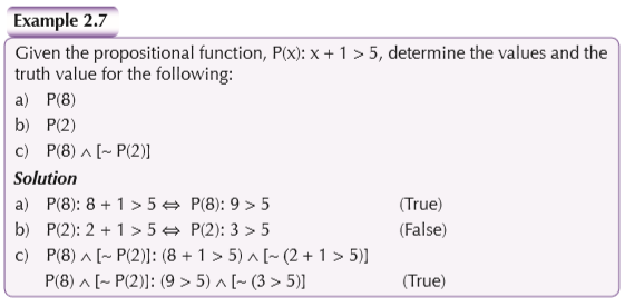
The propositional functions are propositions that contain variables i.e. a sentence expressed in a way that would assume the value of true or false, except that within the sentence there is a variable (x) that is not defined or specified, which leaves the statement undetermined.
The statements such as x+2 > 5 are declarative statements but not propositions when the variables are not specified. However, one can produce propositions from such statements. A propositional function or predicate is an expression involving one or more variables defined on some domain, called the domain of discourse. Substitution of a particular value for the variable(s) produces a proposition which is either true or false. For instance, P(x) : x+2 > 5 is a predicate on the set of real numbers. Observe that P(2) is false, P(4) is true. In the expression P(x); x is called a free variable. As x varies, the truth value of P(x) varies as well. The set of true values of a predicate P(x) is called the truth set.
Activity 2.4
Carry out research to find the meaning of a propositional function. Discuss your findings, using examples, with the rest of the class.
Logic quantifiers
a) Universal quantifier
The universal quantifier is the symbol "∀" read as “for all” or “given any”. It means that each element of a set verifies a given property defined on that set.
For example, consider the following equation in : 1x = x Every x that belongs to , verify the equation. In form of equation we write ∀ x ∈ : 1x = x.
b) Existence quantifier
The symbol “∃” read as “there exists” is called existence quantifier. It means that we can find at least an element of a set which verifies a given property defined on the set.
For example, consider the following inequality in : x + 3 < 5. In this case, x represents a range of elements which verify the inequality. In form of equation we write
∃ x ∈ , x + 3 < 5
The symbol “∃!” read as “there exists only one” is used in the case of unique existence.
Negation of logical quantifiers
Activity 2.5
In groups, consider the statement:
p: All students in this class are brown
Discuss what is required to show the statement is false by explaining and thus negate the statement.
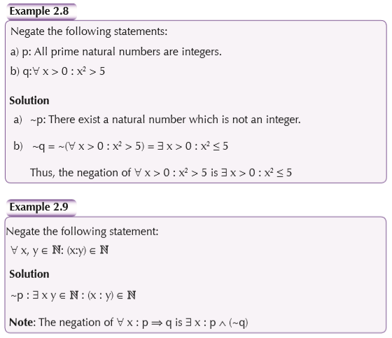
The negation of ‘All students in this class are boys’ is ‘There is a student in this class who is not a boy’.
To negate a statement with a universal quantifier, we change a universal quantifier to the existential one and then negate the propositional function, and vice versa.
The negation of ∀ x : p is ∃ x : (~p) and the negation of ∃ x : p is ∀ x : (~p) and thus:
~ (∀ x : p) ≡ ∃ x : (~p))
~ (∃ x : p) ≡ ∀ x : (~p)
2.4 Applications
Activity 2.6
In pairs, carry out research on the different ways we can apply propositional and predicate logic. Discuss your findings with the rest of the class.
Set theory
Activity 2.7
Carry out research to answer the following:
What is set theory?
How is it an application in logic?
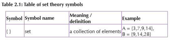
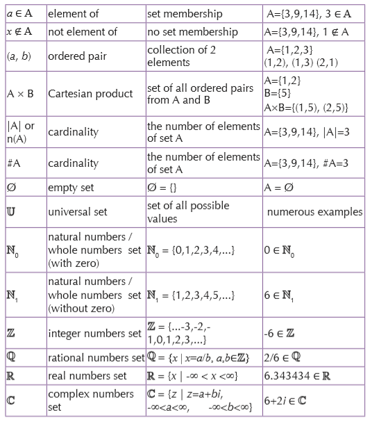
Set theory is the branch of mathematical logic that studies sets, which informally are collections of objects. Although any type of object can be collected into a set, set theory is applied most often to objects that are relevant to mathematics.
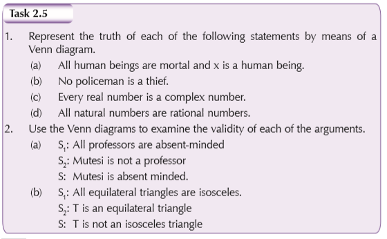
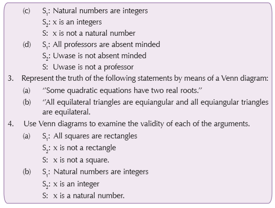
In logic, Venn diagrams can be used to represent the truth of certain statements and also for examining logical equivalence of two or more than two statements.

Electric circuits
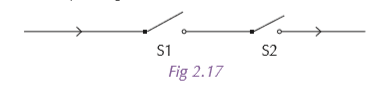
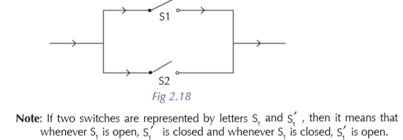
If in an electric network two switches are used, then the two switches S1 and S2 can be in one of the following two cases;
• In series: then the current will flow through the circuit only when the two switches S1 and S2 are on (i.e. closed).
• In parallel: the current will flow through the circuit if and only if either S1 or S2 or both are on (i.e. closed)
Equivalent circuits
Two circuits involving switches S1, S2, …, are said to be equivalent if for every positions of the switches, either current passes through both the circuits, or it does not pass through either circuit.
UNIT 3 : Binary operations
Key unit competence
Use mathematical logic to understand and perform operations using the properties of algebraic structures.
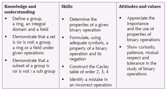
Learning objectives
3.1 Introduction
Activity 3.1
Work in groups.
1. Discuss what you understand by the term binary operations.
2. Carry out research to find the meaning as used in mathematics.
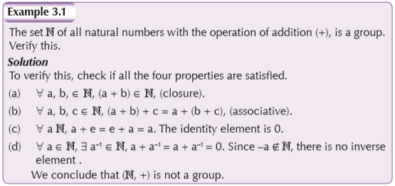
In mathematics, a binary operation on a set is a calculation that combines two elements of the set (called operands) to produce another element of the set. Typical examples of binary operations are the addition (+) and multiplication (×) of numbers and matrices as well as composition of functions on a single set. For example:
• On the set of real numbers , f(a, b) = a × b is a binary operation since the sum of two real numbers is a real number.
• On the set of natural numbers , f(a, b) = a + b is a binary operation since the multiplication of two natural numbers is a natural number. This is a different binary operation than the previous one since the sets are different.
3.2 Groups and rings
Activity 3.2
Work in groups.
1. Discuss what you understand by the terms binary, group, ring, integral domain and field.
2. Carry out research to find their meanings as used in mathematics.
Group
A group (G,*) is a non-empty set (G) on which a given binary operation (*) is defined such that the following properties are satisfied:
(a) Closure property: ∀ a, b ∈ G, (a * b) ∈ G.
(b) Associative property: ∀ a, b, c ∈ G, a * (b * c) = (a* b) *c
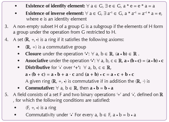
(c) Identity property: ∀ a ∈ G, ∃ e ∈ G, a * e = e * a = a
(d) Inverse element property : ∀ a ∈ G, ∃ a–1 ∈ G, a * a–1 = a–1 * a = e, where e is an identity element.
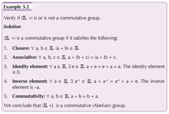
A group is commutative (Abelian) if in addition to the previous axioms, it satisfies commutativity: ∀ a, b ∈ G, a * b = b * a
Subgroups
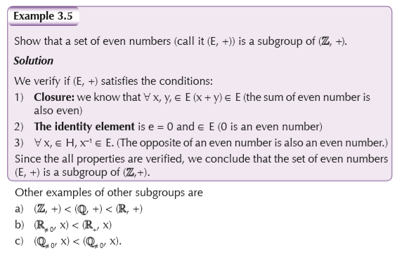
A non-empty subset H of a group G is a subgroup if the elements of H form a group under the operation from G restricted to H. The entire group is a subgroup of itself and is called the improper subgroup.
Every group has a subgroup consisting of an identity element alone and is called the trivial subgroup. The identity element is an element of every subgroup of a group.
If H ≠ G, we call it a subgroup H of G; proper, and we write H < G.
If H ≠ {e}, we call it a subgroup H of G; nontrivial, and we write H ≤ G.
(H, ) is a subgroup of (G, ) if it verifies the following conditions:
1) Closure: ∀ x, y, ∈ H, (x y) ∈ H
2) e ∈ H
3) ∀ x, ∈ H, x–1 ∈ H
where e is the identity element and x–1 is the inverse of x.
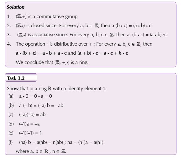
Rings
3.3 Fields and integral domains
Fields
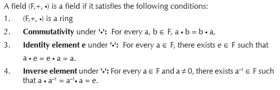
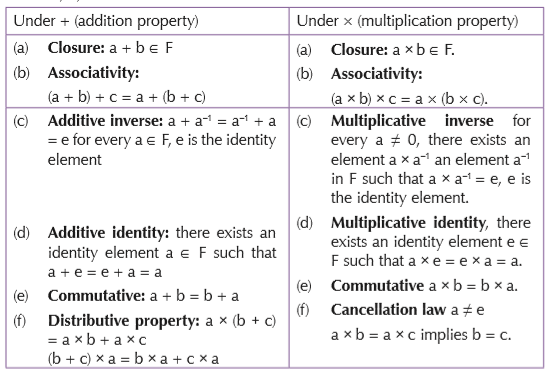
A field F is a non-empty set defined by the following properties. For all a, b, c ∈ F:
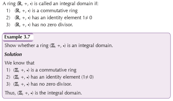
Integral domain
An integral domain is a commutative ring with an identity (1≠ 0) with no zerodivisors. That is ab = 0 ⇒ a = 0 or b = 0.
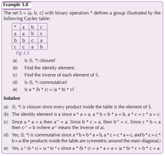
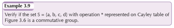
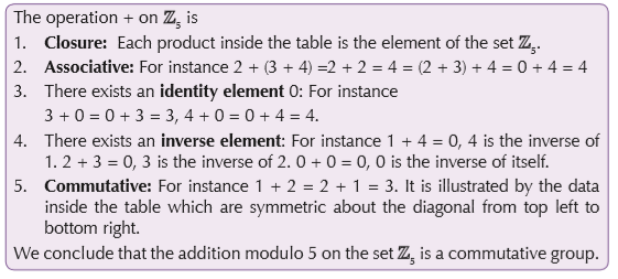
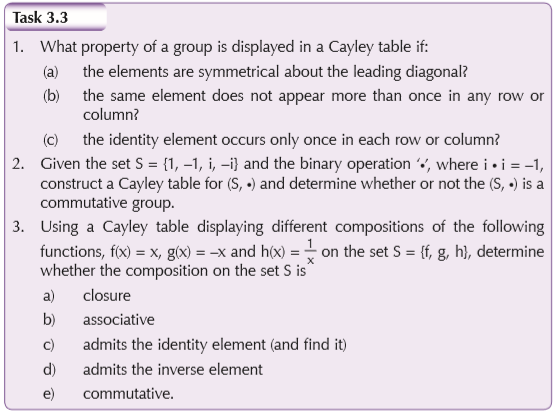
3.4 Cayley tables
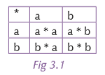
A Cayley table is a useful device for studying binary operations on finite sets. It can be used to help determine if the set under a given operation is a group or not. Given a binary operation (S, *), with S a finite set, its Cayley table has the elements of S listed in the top row and left hand column of the table, and inside the table we write the outcome a * b of the operation in the row labelled with a and the column labelled with b. The elements should be placed along the top row and the left side column in the same order. The following illustrates the Cayley table of the set S = {a, b} under the operation *:
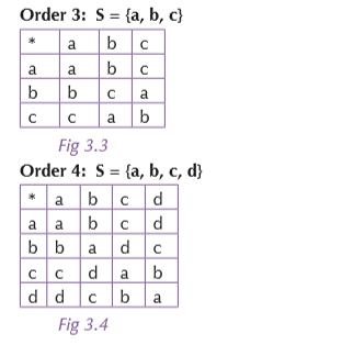
Below we use Cayley tables to illustrate the groups of order 2, 3 and 4.
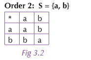
We remark that a * a = a, a * b = b, b * a = b, and b * b = a
We can use Cayley tables to determine if (S, *) is closed, commutative, admits identity element or inverse element.
Closure: If all elements inside the table are in the original set S, then (S, *) is closure.
Commutative: The Cayley table is symmetric about the diagonal. This will only happen if every corresponding row and column are identical.
Identity: In a Cayley table, the identity element is the one that leaves all elements of the set S unchanged.
Inverse: It is found by asking: ‘’What other element can I combine with this one to get the identity?’’
Associative: It is checked by simply respecting the rules of parentheses in comparing if the two sides are equal.
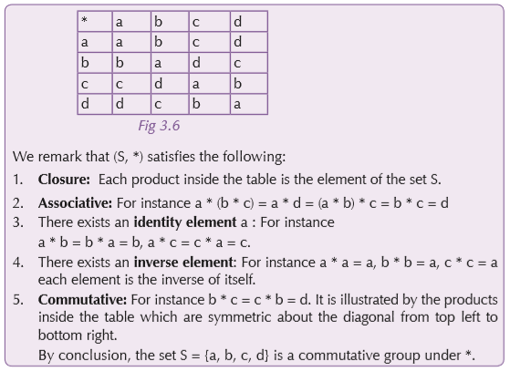
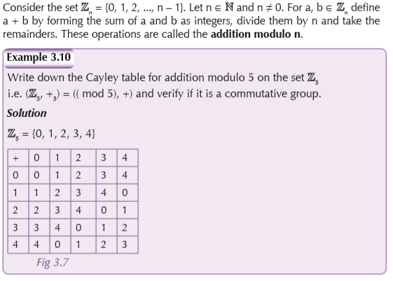
Modular arithmetic

UNIT 4 : Set lR of real numbers
Key unit competence
Think critically using mathematical logic to understand and perform operations on the set of real numbers and its subsets using the properties of algebraic structures.
Learning objectives
4.1 Introduction
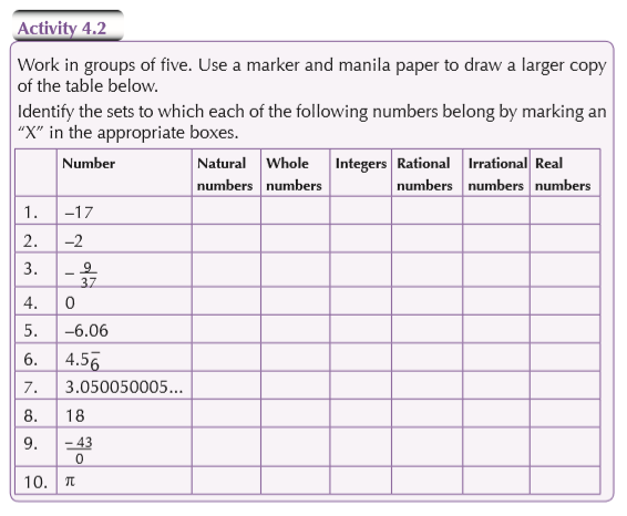
Activity 4.1
Work in groups.
1. Discuss the following: What are sets? What are real numbers?
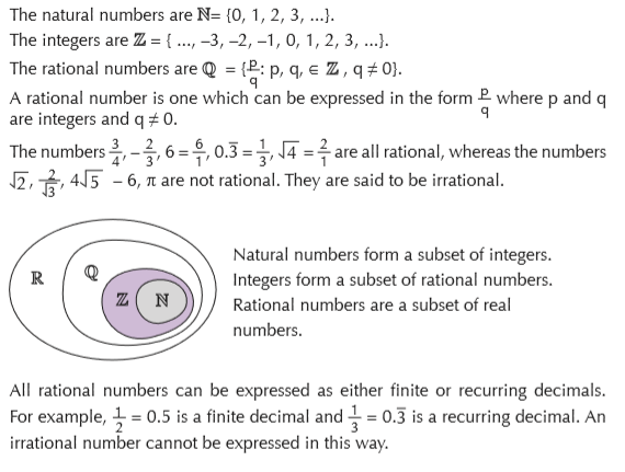
2. Carry out research on sets of numbers to determine the meanings of natural numbers, integers, rational numbers and irrational numbers.

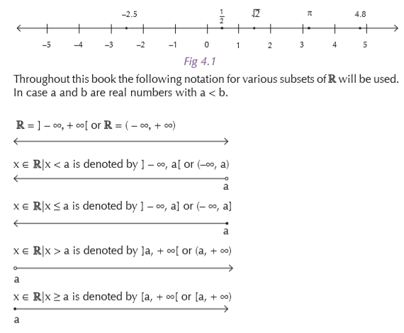
The one-to-one correspondence between the real numbers and the points on the number line is familiar to us all. Corresponding to each real number there is exactly one point on the line: corresponding to each point on the line there is exactly one real number.
4.2 Properties of real numbers
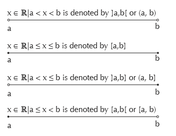
Subsets of real numbers

Order properties
If a and b are any two real numbers, then either a < b or b < a or a = b. The sum and product of any two positive real numbers are both positive.
If a < 0 then (– a) >0.
If a < b then (a – b) > 0. This means that the point on the number line corresponding to a is to the right of the point corresponding to b.
The elementary rules for inequalities are:
1. If a < b and c is any real number then a + c < b + c . That is we may add (or subtract) any real number to (or from) both sides of an inequality.
2. (a) If a < b and c > 0, then ac < bc. (b) If a < b and c < 0, then ac > bc. We may multiply (or divide) both sides of an inequality by a positive real number, but when we multiply (or divide) both sides of an inequality by a negative real number we must change the direction of the inequality sign.
3. (a) If 0 < a < b then 0 < a2 < b2.
(b) If a < b < 0 then a2 > b2. We may square both sides of an inequality if both sides are positive. However if both sides are negative we may square both sides but we must reverse the direction of the inequality sign and then both sides become positive. If one side is positive and the other negative we cannot use the same rule. For example, –2 < 3 and (–2)2 < 32 , but –3 < 2 and (–3)2 > 22.
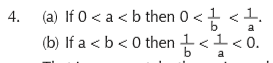
That is we may take the reciprocal of both sides of an inequality only if both sides have the same sign and, in each possible case, we must reverse the direction of the inequality sign.
4.3 Absolute value functions
Activity 4.3
In groups of four, research on the meaning of absolute value. Present your findings to the rest of the class for discussion. Make use of diagrams and examples.
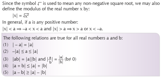
There is a technical definition for absolute value, but you could easily never need it. For now, you should view the absolute value of a number as its distance from zero.
Let us look at the number line.
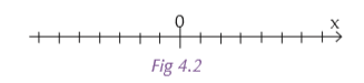
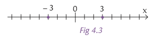
The absolute value of x, denoted "| x |" (and which is read as "the absolute value of x"), is the distance of x from zero. This is why absolute value is never negative; absolute value only asks "how far?", not "in which direction?" This means not only that | 3 | = 3, because 3 is three units to the right of zero, but also that | –3 | = 3, because –3 is three units to the left of zero.
Note: The absolute-value notation is bars, not parentheses or brackets. Use the proper notation. The other notations do not mean the same thing.
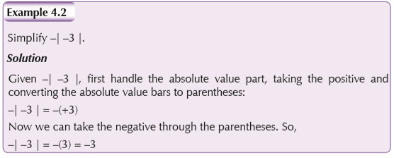
As this illustrates, if you take the negative of an absolute value, you will get a negative number for your answer.
Sometimes we order numbers according to their size. We denote the size or absolute value of the real numbers x by |x|, called the modulus of x.

4.4 Powers and radicals
Powers
Activity 4.4
1. In pairs, revise the meaning of the term 'power'. Give the definition.
2. Research and derive the rules of exponential expressions.
The power of a number says how many times we use the number in a multiplication. It is written as a small number to the right and above the base number. Another name for power is index or exponent.
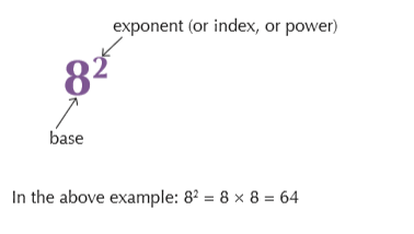
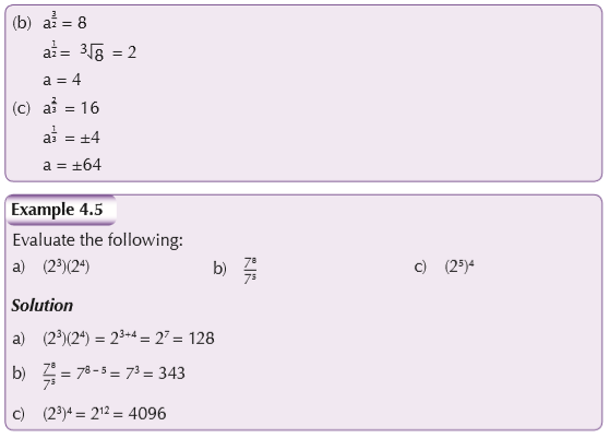
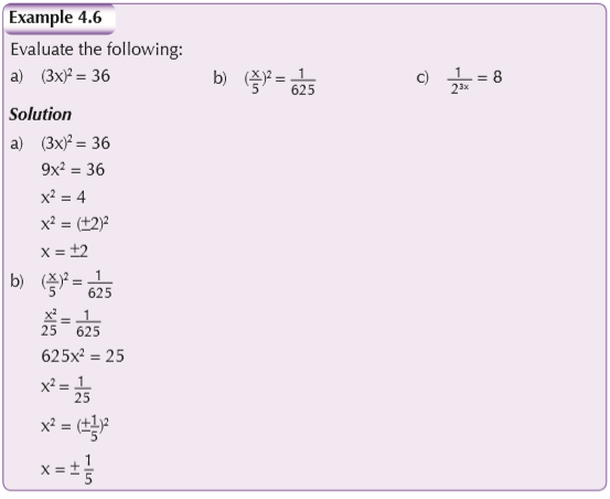
When a real number a is raised to the index m to give am , the result is a power of a. When am is formed, m is sometimes called the power, but it is more correctly called the index to which a is raised.
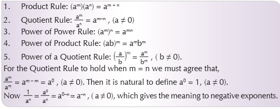
The rules used to manipulate exponential expressions should already be familiar with the reader. These rules may be summarized as follows:
Rational exponents
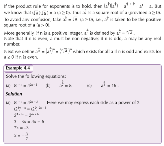
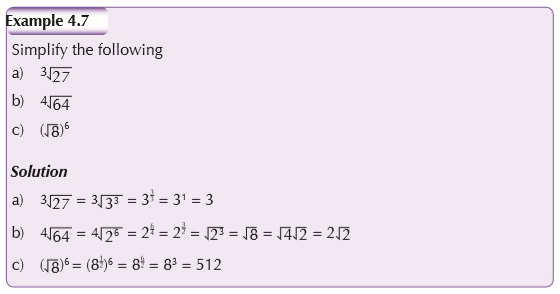
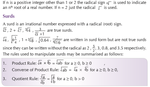
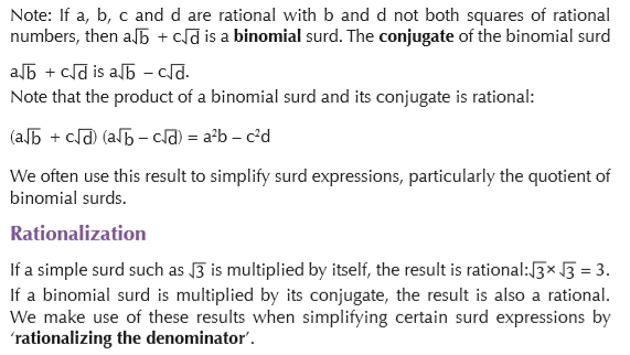
Radicals
Activity 4.5
Research on the meaning of the term radical. Discuss your findings with the rest of the class. Your teacher will assist you get a concise meaning of the term.

2. Every positive number has two square roots, one of which is positive and the other negative.
3. The square root of zero is zero.
4. Negative real numbers have no real square roots.
Cube roots
If a3 = b, then b is the cube of a and a is the cube root of b. This time we say the cube root of b since 23 = 8 but (–2)3 = –8.
1. No definition is needed to specify which cube root is meant since a real number has one and only one cube root in the real number system.
2. Every positive number has one and only one cube root which is positive.
3. The cube root of zero is zero.
4. Every negative number has one and only one cube root which is negative.
Nth roots
In general, if n is an even positive integer then in the real number system:
1. If a > 0, a has two nth roots, one positive and another negative.
2. If a = 0, a has one nth root which is zero.
3. If a < 0, a has no real nth roots.
If n is an odd positive integer (not 1) then in the real number system,
1. If a > 0, a has one nth root which is positive.
2. If a = 0, a has one nth root which is zero.
3. If a < 0, a has one nth root which is negative.
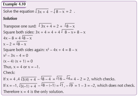
Irrational equations
The process of squaring both sides is used in solving irrational equations, i.e., equations involving surd expressions. It is therefore always necessary to check any solution obtained.
4.5 Decimal logarithms
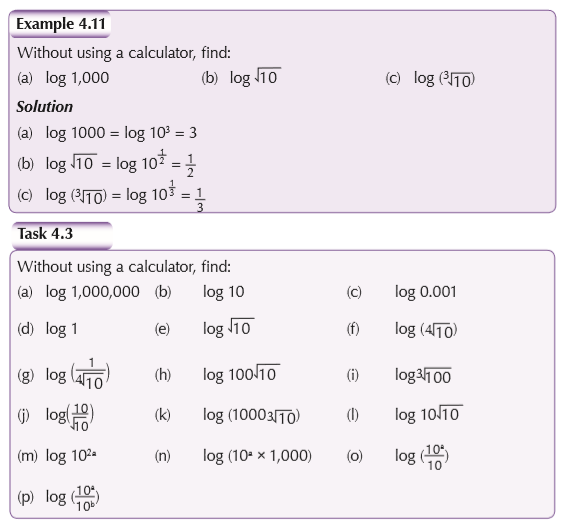
Activity 4.6
Discuss in groups of four and give two examples for each.
1. What is a decimal?
2. What is a logarithm?
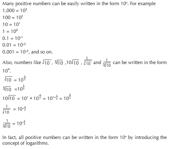
Definition
The logarithm of a positive number, in base 10, is its power of 10. For instance:
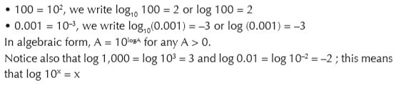
Note: If no base is indicated we assume that it is base 10.
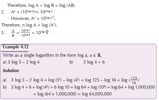
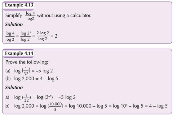
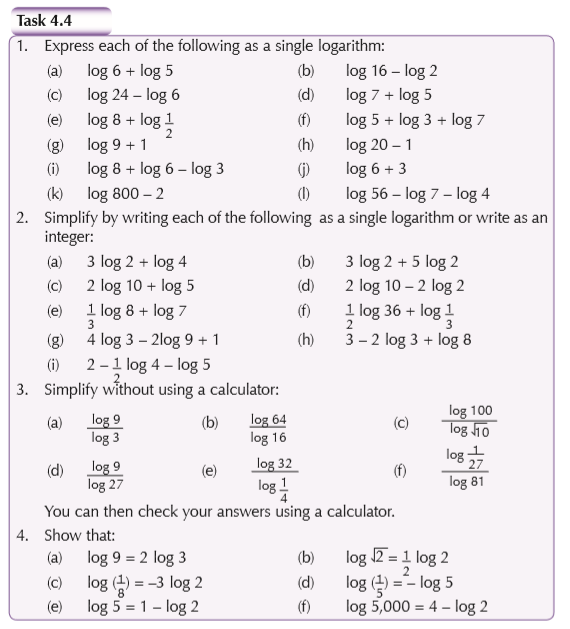
The laws of logarithms
Activity 4.7
Your teacher will guide you in deriving the laws of logarithms. Use numerous examples to practise using them.
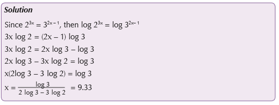
The logarithm can be used in solving exponential equations.
Application of exponents in real life
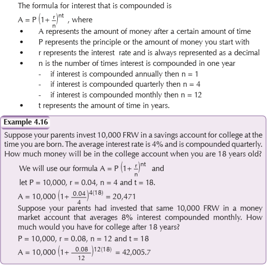
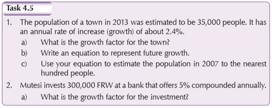
Compound interest
UNIT 5 : Linear equations and inequalities
Key unit competenceModel and solve algebraically or graphically daily life problems using linear equations or inequalities.
Learning objectives
5.1 Equations and inequalities in one unknown
In Junior Secondary, we learnt about linear equations and inequalities.
Activity 5.1
Research on the following:
1. What is a linear equation?
2. What is a linear inequality?
Present your findings, with clear examples, to the rest of the class.
Linear equations
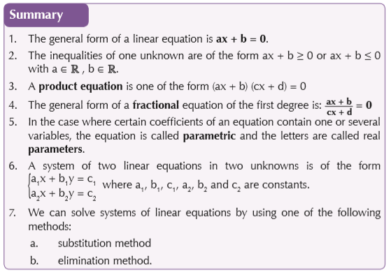
A linear equation is an equation of a straight line. For example:

Solving linear equations
• A linear equation is a polynomial of degree 1.
• In order to solve for the unknown variable, you must isolate the variable.
• In the order of operation, multiplication and division are completed before addition and subtraction.

Activity 5.2
Discuss in groups and verify that the following are true.
Product equation
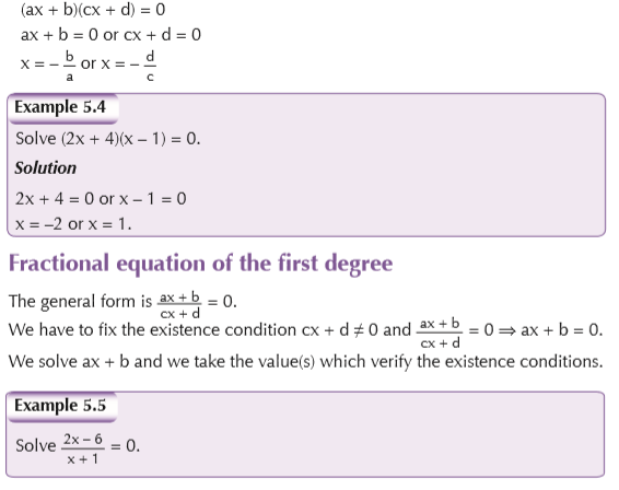
This is in the form (ax + b)(cx + d) = 0.
Since the product of factors is null (zero) either one of them is zero. To solve this we proceed as follows:
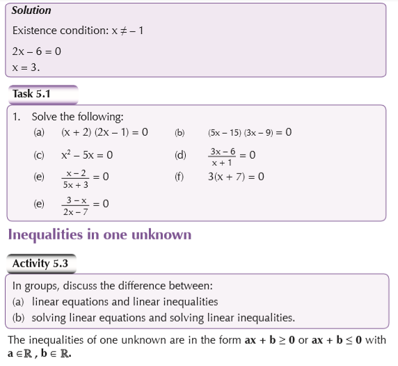
Solving inequalities
They are solved as linear equations except that:
(a) when we multiply an inequality by a negative real number the sign will be reversed
(b) when we interchange the right side and the left side, the sign will be reversed.

Graphs
The graph of a linear inequality in one variable is a number line. We use an unshaded circle for < and > and a shaded circle for ≤ and ≥. The graph for x > –3:

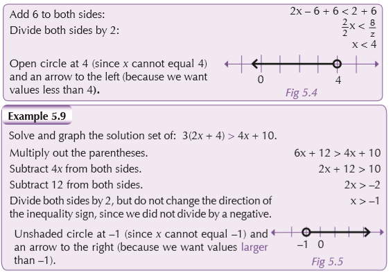
Figure 5.6 shows a graph of a linear inequality.
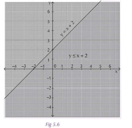
The inequality is y ≤ x + 2.
You can see the line, y = x + 2 and the shaded area is where y is less than or equal to x + 2
5.2 Parametric equations and inequalities
Activity 5.4
Carry out research. Find the meaning of parametric equations and inequalities. Discuss your findings using suitable examples.
Parametric equations
There are also a great many curves that we cannot even write down as a single equation in terms of only x and y. So, to deal with some of these problems we introduce parametric equations. Instead of defining y in terms of x i.e y = f(x)) or x in terms of y i.e x = h
we define both x and y in terms of a third variable called a parameter as follows:
This third variable is usually denoted by t (but does not have to be). Sometimes we will restrict the values of t that we shall use and at other times we will not. If the coefficients of an equation contain one or several letters (variables) the equation is called parametric and the letters are called real parameters. In this case, we solve and discuss the equation (for parameters only).
Each value of t defines a point (x, y) = (f(t),g(t)) that we can plot. The collection of points that we get by letting t be all possible values is the graph of the parametric equations and is called the parametric curve.

Graphs
Sketching a parametric curve is not always an easy thing to do. Let us look at an example to see one way of sketching a parametric curve. This example will also illustrate why this method is usually not the best.
Activity 5.5
In groups of five, work out the following.
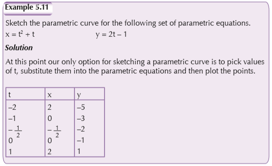
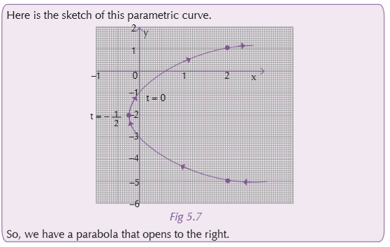
1. Sketch the parametric curve for the following set of parametric equations.
x = t2 + t y = 2t – 1 –1 ≤ t ≤1
2. Eliminate the parameter from the following set of parametric equations.
x = t2 + t y = 2t – 1
3. Sketch the parametric curve for the following set of parametric equations. Clearly indicate the direction of motion.
x = 5 cost y = 2 sin t 0 ≤ t ≤ 2π
Parametric inequalities in one unknown

5.3 Simultaneous equations in two unknowns
Mental task
What are simultaneous linear equations? How do we solve them?
A linear equation in two variables x and y is an equation of the form
We say that we have two simultaneous linear equation in two unknowns or a system of two linear equation in two unknowns.
The pair (x, y) satisfying both equations is the solution of the given equation.
We can solve such systems of linear equations by using one of the following methods:
1. substitution method
2. elimination method.
Substitution
This method is used when one of the variables is given in terms of the other.
Elimination
Elimination method is used to solve simultaneous equations where neither variable is given as the subject of another.

5.4 Applications
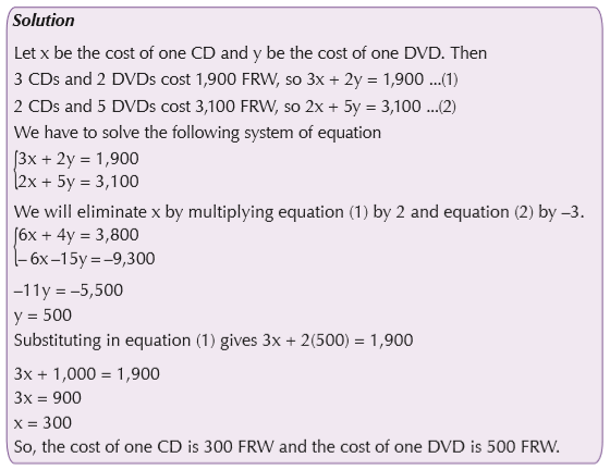
Systems of two equations have a wide practical application whenever decisions arise. Decisions of this nature always involve two unknown quantities or variables. The following steps are hereby recommended in order to apply simultaneous equations for practical purposes.
1. Define variables for the two unknown quantities, in case they are not given.
2. Formulate equations using the unknown variables and the corresponding data.
3. Solve the equations simultaneously.

Activity 5.6
Linear equations and inequalities have their use in our everyday life. Research on these and present your findings for discussion in class.
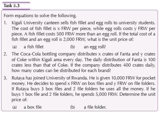
Distance = rate × time
In this equation, for any given steady rate, the relationship between distance and time will be linear. However, distance is usually expressed as a positive number, so most graphs of this relationship will only show points in the first quadrant. Notice that the direction of the line in the graph of Figure 5.8 is from bottom left to top right. Lines that tend in this direction have positive slope. A positive slope indicates that the values on both axes are increasing from left to right.
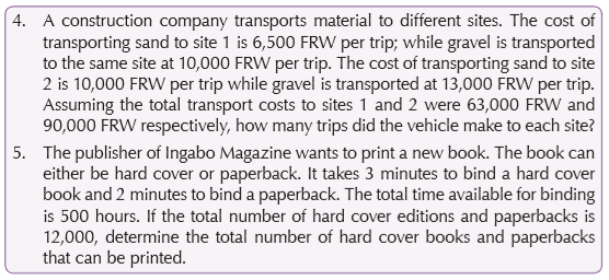
Amount of water in a leaking bucket = rate of leak × time
In this equation, since you cannot have a negative amount of water in the bucket, the graph will also show points only in the first quadrant. Notice that the direction of the line in this graph is top left to bottom right. Lines that tend in this direction have negative slope. A negative slope indicates that the values on the y axis are decreasing as the values on the x axis are increasing.
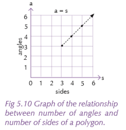
Number of angles of a polygon = number of sides of that polygon
In this graph, we are relating values that only make sense if they are positive, so we show points only in the first quadrant. In this case, since no polygon has fewer than 3 sides or angles, and since the number of sides or angles of a polygon must be a whole number, we show the graph starting at (3,3) and indicate with a dashed line that points between those plotted are not relevant to the problem.
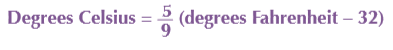
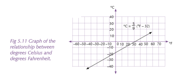
Since it is perfectly reasonable to have both positive and negative temperatures, we plot the points on this graph on the full coordinate grid.
UNIT 6 : Quadratic equations and inequalities
Key unit competence
Model and solve algebraically or graphically daily life problems using quadratic equations or inequalities.
Learning objectives
6.1 Introduction
In Senior 3, we learnt about quadratic equations and ways to solve them.
Activity 6.1
Carry out research to obtain the definition of quadratic equation. Discuss your findings with the rest of the class.
The term quadratic comes from the word quad meaning square, because the variable gets squared (like x2). It is also called an “equation of degree 2” because of the “2” on the x.
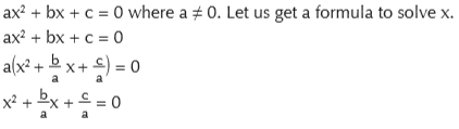
The standard form of a quadratic equation looks like this: ax2 + bx + c = 0
where a, b and c are known values and a cannot be 0.
“x” is the variable or the unknown.
Here are some more examples of quadratic equations:
2x2 + 5x + 3 = 0 In this one, a = 2, b = 5 and c = 3
x2 − 3x = 0 For this, a = 1, b = –3 and c = 0, so 1 is not shown.
5x − 3 = 0 This one is not a quadratic equation. It is missing a value in x2 i.e a = 0, which means it cannot be quadratic.
6.2 Equations in one unknown
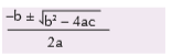
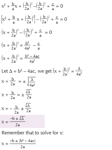
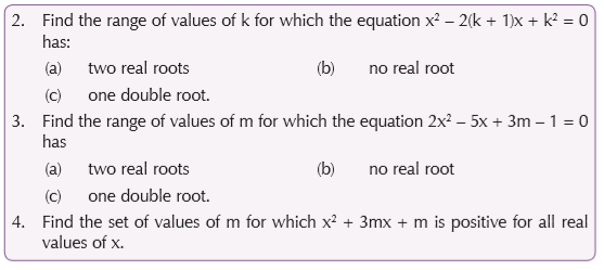
A quadratic equation in the unknown x is an equation of the form ax2 + bx + c = 0, where a, b and c are given real numbers, with a ≠ 0. This may be solved by completing the square or by using the formula
• If b2 – 4ac > 0, there are two distinct real roots
• If b2 – 4ac = 0, there is a single real root (which may be convenient to treat as two equal or coincident roots)
• If b2 – 4ac < 0, the equation has no real roots.
We know that the quadratic equation is of the form:
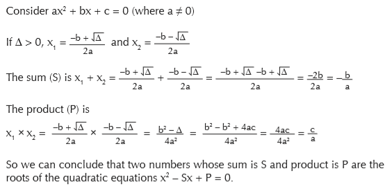
Sum and product of roots
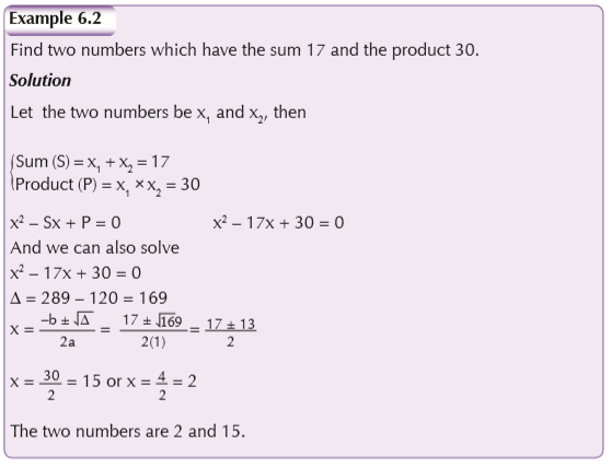
Activity 6.2
In pairs, form the quadratic equations that have 7 and –3 as roots.
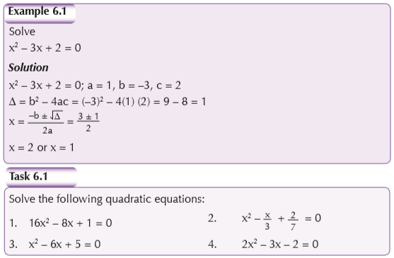
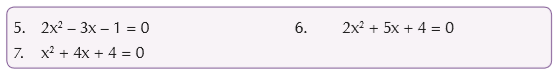
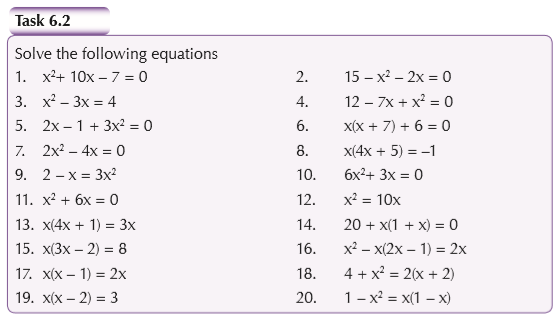
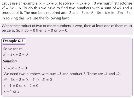
Solving quadratic equations by factorizing

6.3 Inequalities in one unknown
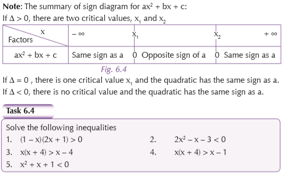
The product ab of two factors is positive if and only if
(i) a > 0 and b > 0 or
(ii) a < 0 and b < 0.
Sign diagrams
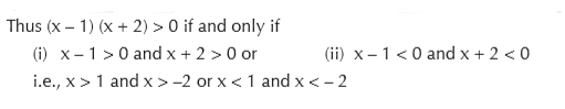
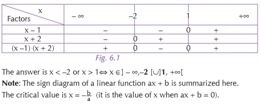
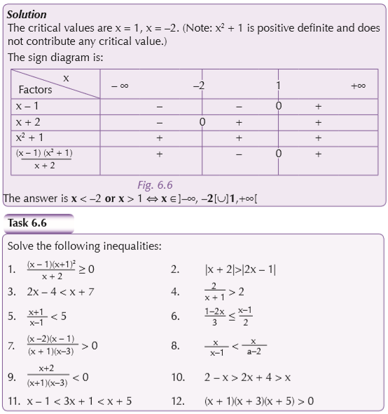
Although this method is sound it is not of much practical use in more complicated problems. A better method which is useful in more complicated problems is the following which uses the ‘’sign diagram’’ of the product (x – 1)(x + 2).
(x – 1) (x + 2) > 0
The critical values are x = 1 and x = –2. (i.e., the values of x at which the factor is zero.)
The sign diagram of (x – 1) (x + 2) is thus:

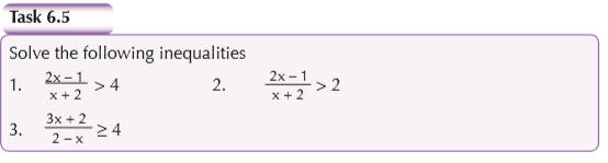
Inequalities depending on the quotient of two linear factors

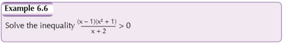
Solving general inequalities
The techniques illustrated in the previous pages can be used to solve complicated inequalities. There are also other techniques which may be used in special cases.
6.4 Parametric equations
In case certain coefficients of equations contain one or several letter variables, the equation is called parametric and the letters are called real parameters. In this case, we solve and discuss the equation (for parameters only).

Parametric equations in one unknown
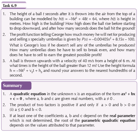
If at least one of the coefficients a, b and c depend on the real parameter which is not determined, the root of the parametric quadratic equation depends on the values attributed to that parameter
6.5 Simultaneous equations in two unknowns
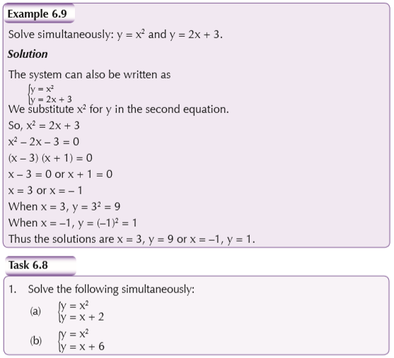
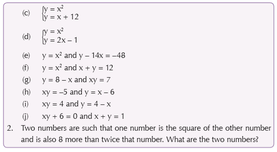
To solve simultaneous equations involving a quadratic equation we use substitution of one equation into the other.
6.6 Applications of quadratic equations and inequalities
Activity 6.3
In groups of five, research on the importance and necessity of quadratic equations and inequalities.
Quadratic equations lend themselves to modelling situations that happen in real life. These include:
• projectile motions
• the rise and fall of profits from selling goods
• the decrease and increase in the amount of time it takes to run a kilometre based on your age, and so on.
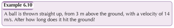
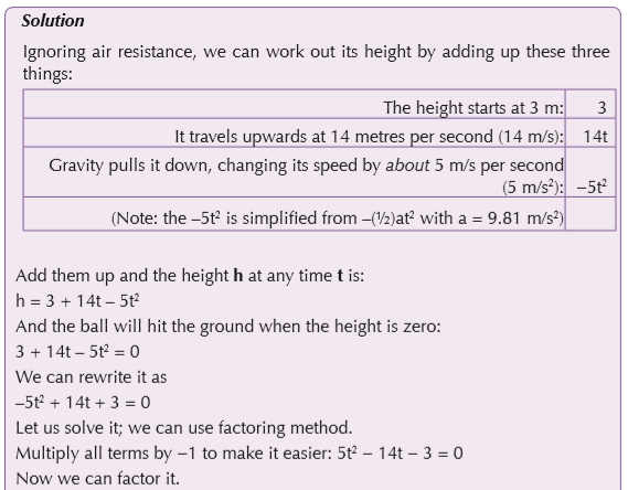
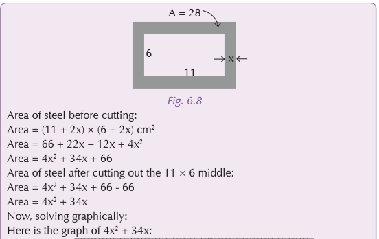
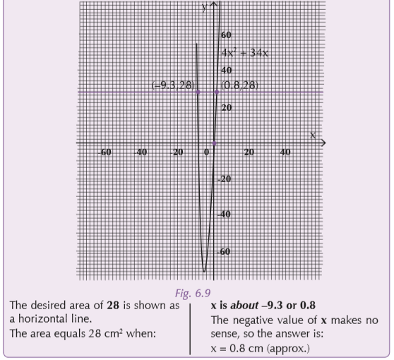
The wonderful part of having something that can be modelled by a quadratic is that you can easily solve the equation when set equal to zero and predict. If you throw a ball (or shoot an arrow, fire a missile or throw a stone) it will go up into the air, slowing down as it goes, then come down again. A quadratic equation can tell you where it will be at any given time.

UNIT 7 : Polynomial, rational and irrational functions
Key unit competence
Use concepts and definitions of functions to determine the domain of rational functions and represent them graphically in simple cases and solve related problems.
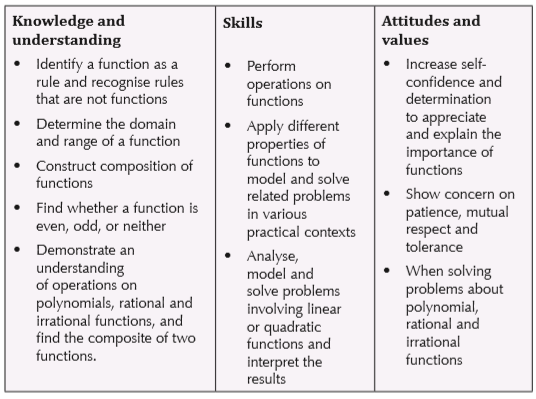
Learning objectives
7.1 Polynomials
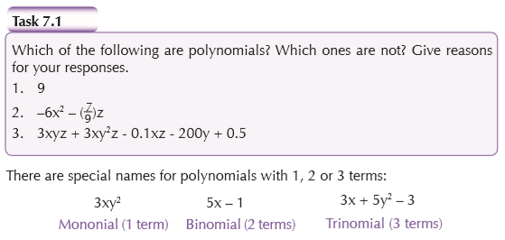
Activity 7.1
Research on the definition of polynomial. Discuss with the rest of the class to come up with a concise definition.
Polynomial
comes from poly- meaning “many” and -nomial meaning “term”. A polynomial looks like this:
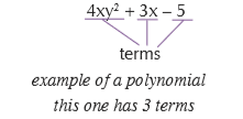
A polynomial can have:
• constants (like 3, –20, or ½)
• variables (like x and y)
• exponents (like the 2 in y2), but only 0, 1, 2, 3, ... etc
that can be combined using addition, subtraction, multiplication and division.
A polynomial can never be divided by a variable such as

Generally

• Polynomials can have no variable at all: For example, 23 is a polynomial. It has just one term, which is a constant.
• Or one variable: For example, x4 – 2x2+x has three terms, but only one variable (x)
• Or two or more variables: For example: xy4 – 5x2z has two terms, and three variables (x, y and z)
The degree of a polynomial with only one variable is the largest exponent of that variable. For example, in 4x3 – x + 3 the degree is 3 the largest exponent of x.
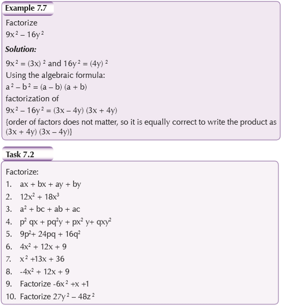
Factorization of polynomials
Activity 7.2
In groups, discuss the meaning of factorization. What are the different operations involved in factorization?
In arithmetic, you are familiar with factorization of integers into prime factors.
For example, 6 = 2 × 3.
The 6 is called the multiple, while 2 and 3 are called its divisors or factors. The process of writing 6 as product of 2 and 3 is called factorization. Factors 2 and 3 cannot be further reduced into other factors.
Like factorization of integers in arithmetic, we have factorization of polynomials into other irreducible polynomials in algebra.
For example, x2 + 2x is a polynomial. It can be factorized into x and (x + 2). x2 + 2x = x (x + 2).
So, x and x + 2 are two factors of x2 + 2x. While x is a monomial factor, x + 2 is a binomial factor.
Factorization is a way of writing a polynomial as a product of two or more factors. Here is an example:
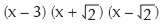
x3 – 3x2 – 2x + 6 = (x – 3) (x2 – 2) =
Types of factorization
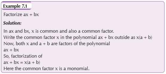
1. Factorization into monomials
Remember the distributive property? It is a (b + c ) = ab + ac
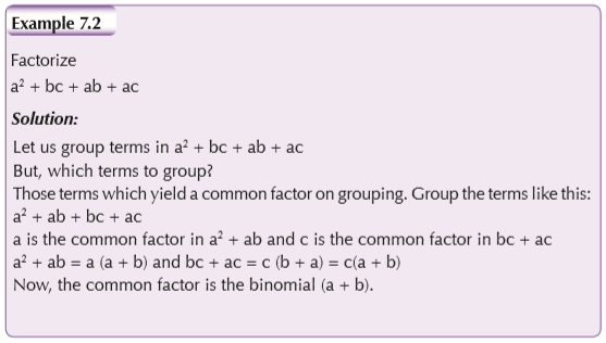
2. By grouping of terms
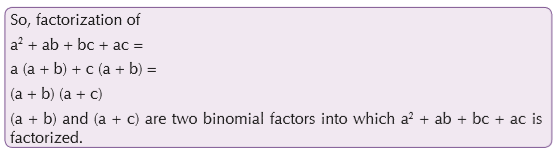
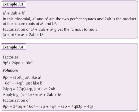
3. Factorization of trinomial perfect squares
Trinomial perfect squares have three monomials, in which two terms are perfect squares and one term is the product of the square roots of the two terms which are perfect squares
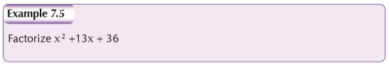
4. Factorization of trinomials of the form x2 + bx + c
5. Factorization of trinomials of the form ax 2 + bx + c

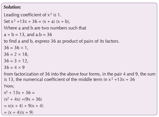
6. Factorization of difference of two perfect squares
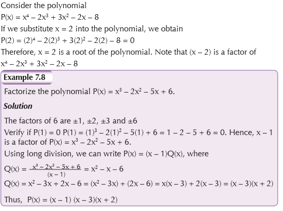
Roots of polynomials
We say that x = a is a root or zero of a polynomial P(x) if it is a solution to the equation P(x) = 0. In other words, x = a is a root of a polynomial P(x) if P(a) = 0. In that case x – a is one of the factors of the polynomial P(x).
7.2 Numerical functions
Definition
Consider two sets A and B. A function from A into B is a rule which assigns a unique element of A exactly one element of B. We write the function from A to B as f: A → B. Most of time we do not indicate the two sets and we simply write y = f(x).
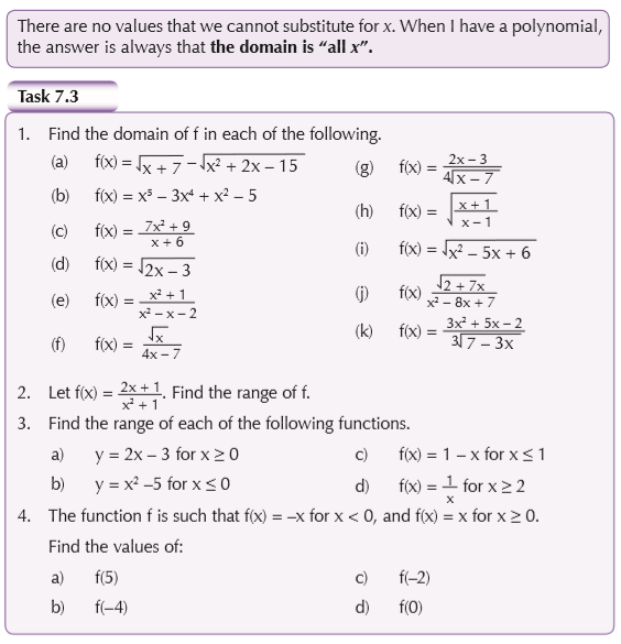
The sets A and B are called the domain and range of f, respectively. The domain of f is denoted by dom (f).
Domain and range of a function
We have been introduced to functions. These involve the relationship or rule connecting domains to ranges.
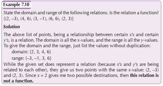
Note that we have to check whether the relation is a function by looking for duplicate x-values. If you find a duplicate x-value, then the different y-values mean that you do not have a function.
Domain
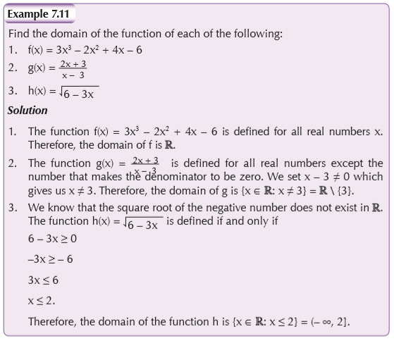
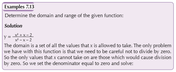
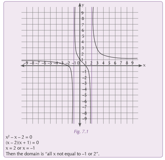
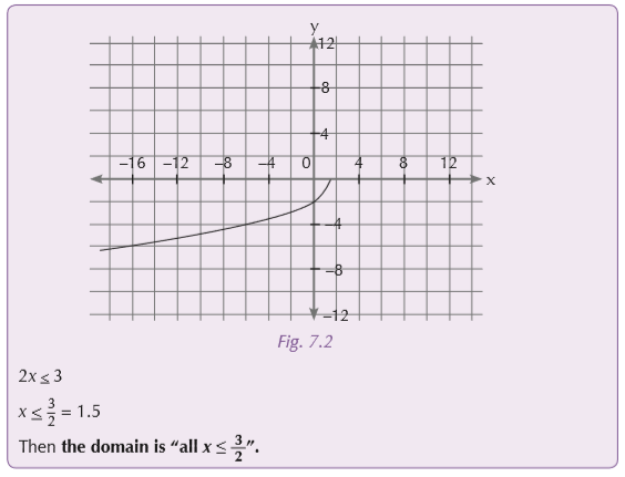
Domain of a function is the set of all real numbers for which the expression of the function is defined as a real number. In other words, it is all the real numbers for which the expression makes sense.
Determination of domain of definition of a function in lR
When determining domain of definition, we have to take into account three things:
• You cannot have a zero in the denominator.
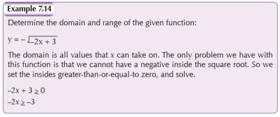
• You cannot have a negative number under an even root.
• You cannot evaluate the logarithm of a negative number
Range
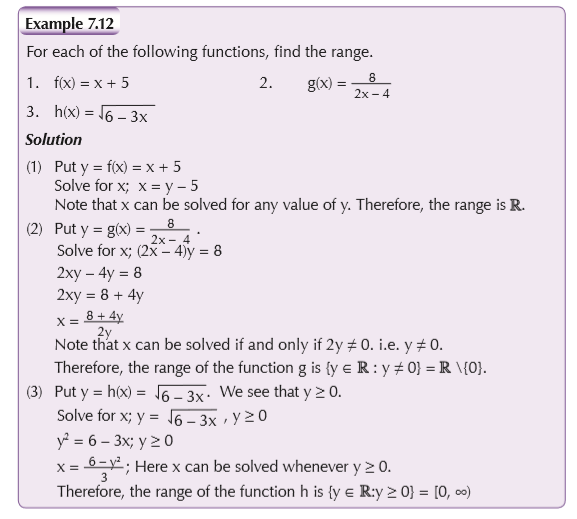
Let f: A → B be a function. The range of f, denoted by Im(f) is the image of A under f, that is, Im (f) = f[A]. The range consists of all possible values the function f can have.
Steps to finding range of function
To find the range of function f described by formula where the domain is taken to be the natural domain:
1. Put y = f(x).
2. Solve x in terms of y
3. The range of f is the set of all real numbers y such that x can be solved.
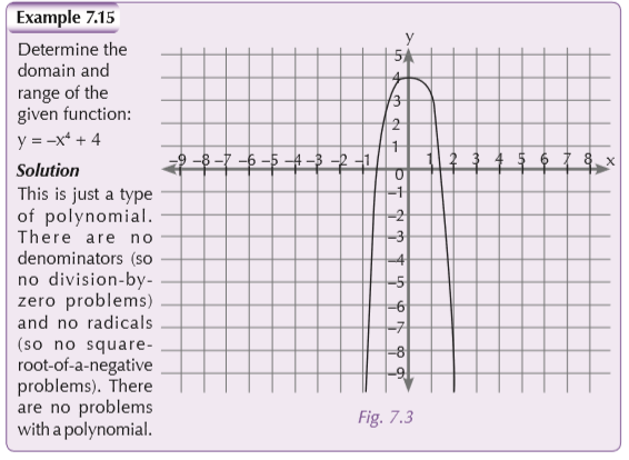
As we can see from, the graph “covers” all y-values (that is, the graph will go as low as I like, and will also go as high as I like). Since the graph will eventually cover all possible values of y, then the range is “all real numbers”.
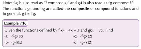
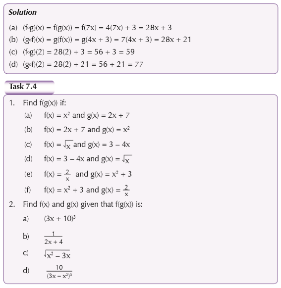
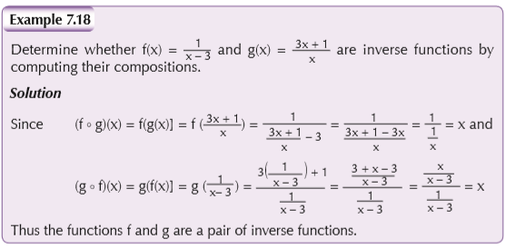
Composition of functions
The composition of g and f, denoted g f is defined by the rule (g f)(x) = g(f(x)) provided that f(x) is in the domain of g.
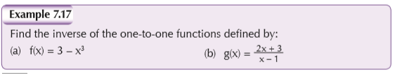
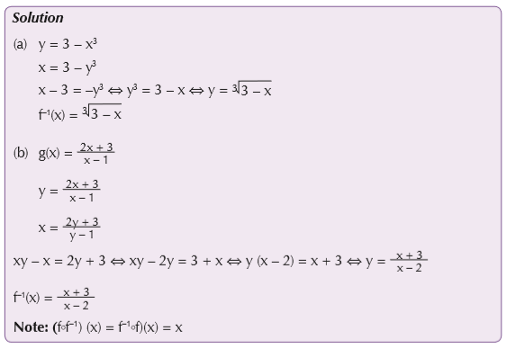
The inverse of a numerical function
For a one-to-one function defined by y = f(x), the equation of the inverse can be found as follows:
I Replace f(x) by y.
II Interchange x and y.
III Solve for y.
IV Replace y by f–1(x)
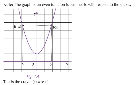
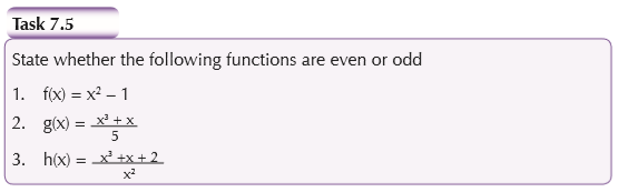
Parity of a function
Even function
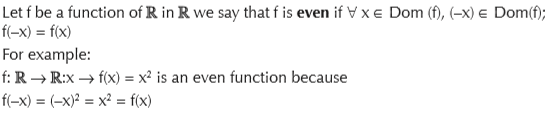
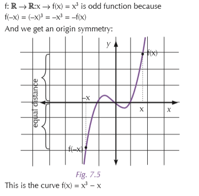
Odd function
We say that a function f is odd if ∀x ∈ Dom (f), (–x) ∈Dom(f);
f(–x) = –f(x)
For example:
7.3 Application of rational and irrational functions
Activity 7.3
In groups of five, research on the different ways of applying functions of rational and irrational number. Discuss your findings in class. Have at least one person from each group demonstrate an example of application to the rest of the class.
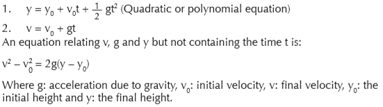
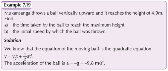
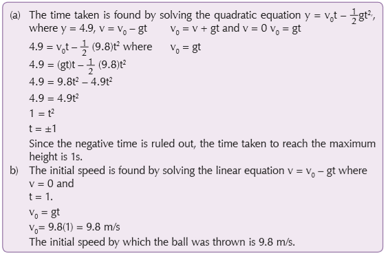
Free falling objects
A free falling object is accelerated toward the earth with a constant acceleration equal to g = 9.8 m/s2. The different formulas used in dealing with free falling objects are:
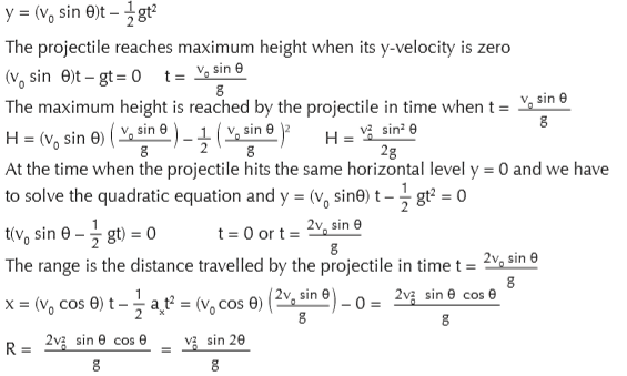
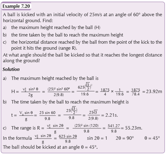
Projectiles
We consider the motion of a projectile fired from ground level at an angle q upward from the horizontal and an initial speed v0. We are interested in finding, how long it takes the projectile to reach the maximum height, the maximum height the projectile reaches and the horizontal distance it travels (called the range, R). In general we use the following formulas:
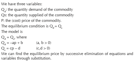
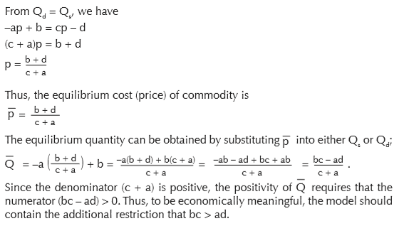
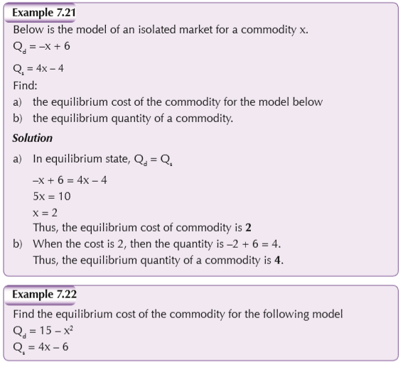
Determination of the equilibrium cost (price) of a commodity in an isolated market
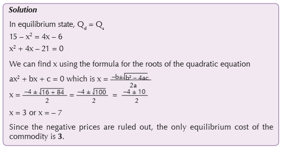
Rates of reaction in chemistry
The rate of reaction of a chemical reaction is the rate at which products are formed. To measure a rate of reaction, we simply need to examine the concentration of one of the products as a function of time.


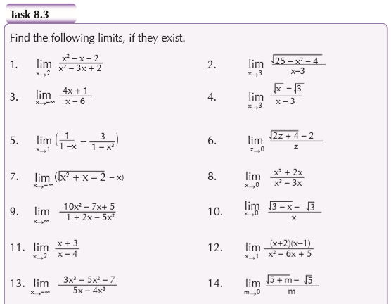
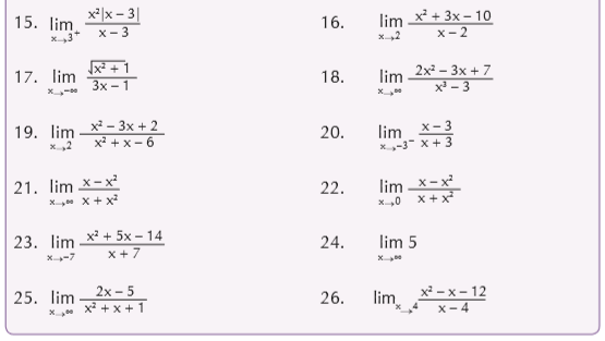
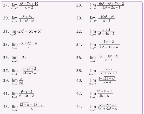
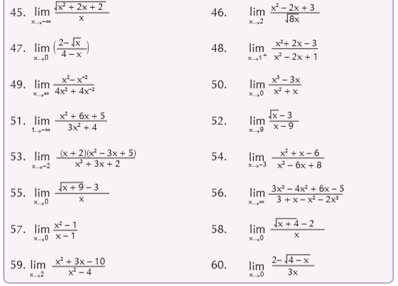
UNIT 8 : Limits of polynomial, rational and irrational functions
Key unit competence
Evaluate correctly limits of functions and apply them to solve related problems.
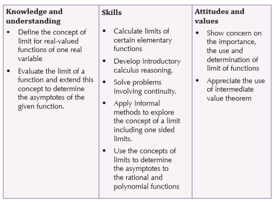
Learning objectives
8.1 Concept of limits
Neighbourhood of a real number
Activity 8.1
You have heard about the term ‘neighbourhood’ in everyday life. What does it mean?
Carry out research to find the meaning of the term in mathematics. Discuss your findings in class. Use diagrams in your explanations.
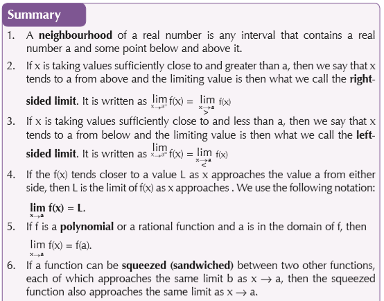
By a neighbourhood of a real number c we mean an interval which contains c as an interior point.
On the real line, a neighborhood of a real number is an open interval (a – δ, a + δ) where δ > 0, with its centre at a. Therefore, we can say that a neighborhood of the real number is any interval that contains a real number a and some point below and above it.
We can add:
Let x be a real number. A neighbourhood of x is a set N such that for some ε > 0 and for all y, if |x − y| < ε then y ∈ N.
Limit of a variable
Activity 8.2
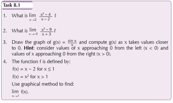
In groups of five, work out the following:
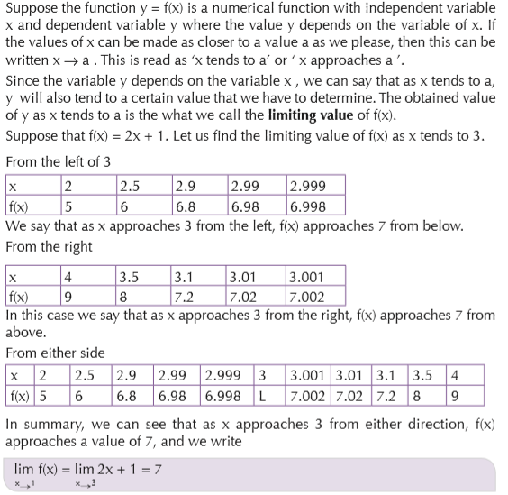
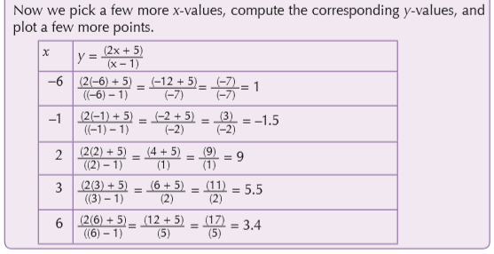
Let f(x) = 2 x + 2 and compute f(x) as x takes values closer to 1. First consider values of x approaching 1 from the left (x < 1) then consider x approaching 1 from the right (x > 1).
In Activity 8.2, x approaching 1 from the left (x < 1) gives us:

and x approaching 1 from the right (x > 1) gives us:
In both cases as x approaches 1, f(x) approaches 4. Intuitively, we say that

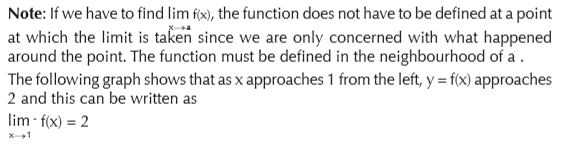
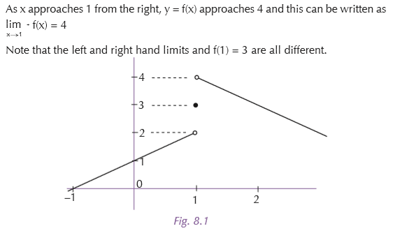
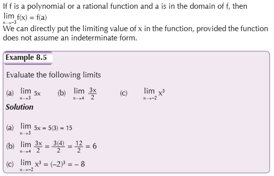
Note: We are talking about the values that f(x) takes when x gets closer to 1 and not f(1). In fact we may talk about the limit of f(x) as x approaches a even when f(a) is undefined.
If f(x) can be made as close as we like to some number a by making x sufficiently close to (but not equal to) a, then we say that f(x) has a limit of L as x approaches a, and we write

Note that in the above case the limit is found by the direct substitution i.e.
One-sided limits
Right-sided limits
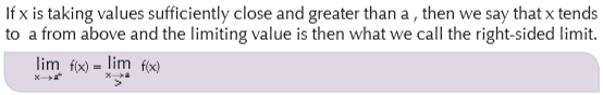
Left-sided limits
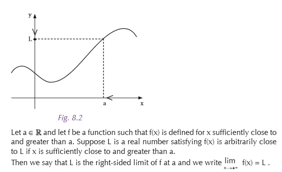
If x is taking values sufficiently close to and less than a, then we say that x tends to a from below and the limiting value is then what we call the left-sided limit. It is written as:
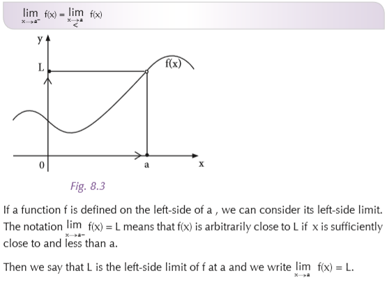
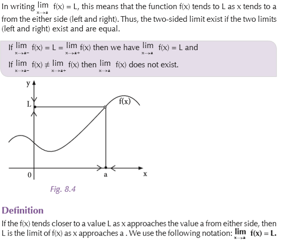
Two-sided limits
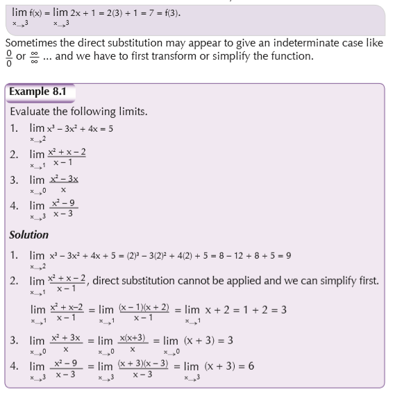
Evaluation of algebraic limits by direct substitution
Infinity limits
Let f be a function defined on both sides of a, except possibly at a itself. Then

means that the values of f(x) can be made arbitrarily large (as large as we please) by taking x
sufficiently close to a, but not equal to a.
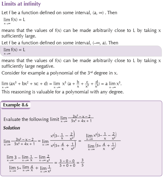
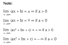
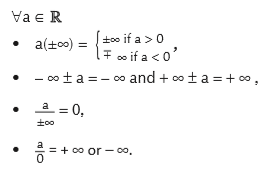
Note: To compute the limit of a function as x → ±∞, we use the following principles
8.2 Theorems on limits
Compatibility with order
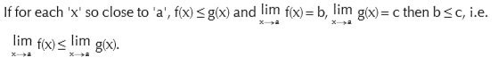
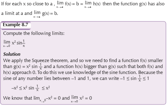
Squeeze theorem
This is also known as the sandwich theorem, comparison theorem or vice theorem. If a function can be squeezed (sandwiched) between two other functions, each of which approaches the same limit b as x → a , then the squeezed function also approaches the same limit as x → a.
Let f(x), g(x) and h(x) be three functions such that f(x) ≤ g(x) ≤h(x).
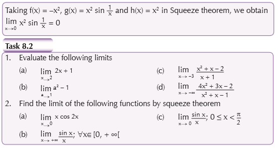
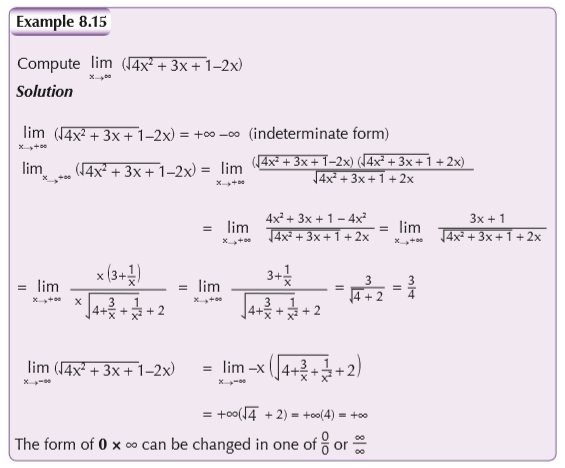
8.3 Indeterminate forms
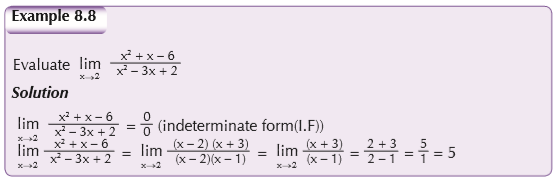
Method of factors

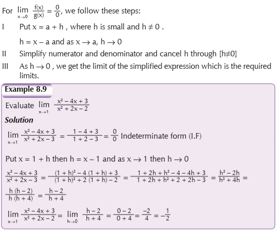
Method of substitution
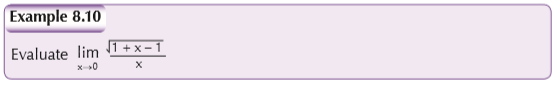
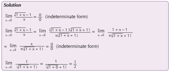
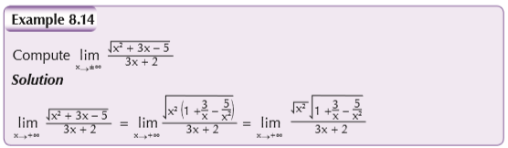
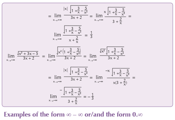
Method of rationalisation
In functions which involve square roots, rationalisation of either numerator or denominator and simplifications will facilitate the work.
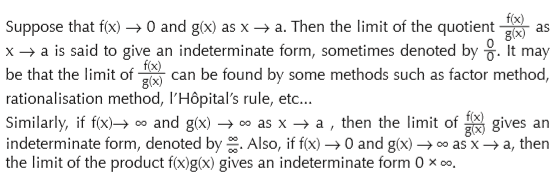
True value of limits
Computation of limits may results in indeterminate form (I.F) such as

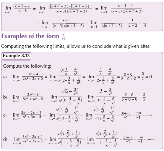
Thus, we we can say that:
• If the degree of the numerator is smaller than the one of the denominator, the limit of the fraction as x → ∞ is zero;
• If the degree of the numerator is equal to the one of the denominator, the limit of the fraction as x → ∞ is equal to the quotient of the coefficient of the terms with the highest power;
• If the degree of the numerator is greater than the one of the denominator, the limit of the fraction as x → ∞ gives infinite (the sign of infinite depends on the highest power and its coefficient).

8.4 Application of limits
Activity 8.4
In groups, carry out research to find out the applications of limits. Discuss your findings with the rest of the class.
Continuity of a function at a point or interval
Points where f fails to be continuous are called discontinuities of f and f is said to be discontinuous at these points.
Continuity over an interval
The function is said to be continuous over interval ]a, b[ if and only if f(x) is continuous at any point of the interval ]a, b[. i.e.
f is continuous for all x0 ∈]a, b[. f is continuous at the right side of a. f is continuous at the left side of b .
Properties1. The sum of two continuous functions is a continuous function.
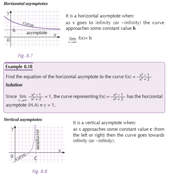
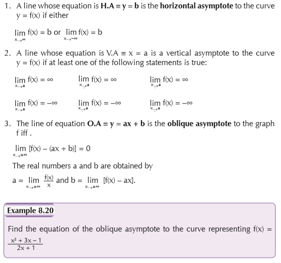
2. The quotient of two continuous functions is a continuous function where the denominator is not zero.Asymptotes
Activity 8.5
What is an asymptote? Carry out research and find out the meaning. Also, find out the types of asymptotes.
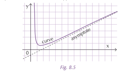
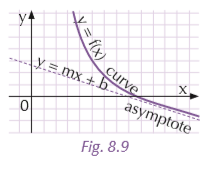
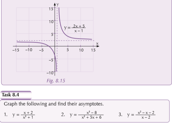
An asymptote is a line that a curve approaches, as it heads towards infinity:
Types
There are three types of asymptotes: horizontal, vertical and oblique:

An asymptote can be in a negative direction, the curve can approach from any side (such as from above or below for a horizontal asymptote), or may actually cross over (possibly many times), and even move away and back again.
The important point is that: The distance between the curve and the asymptote tends to zero as they head to infinity (or−infinity)
Oblique asymptotes
It is an oblique asymptote when: as x goes to infinity (or −infinity) then the curve goes towards a line y = mx + b
(note: m is not zero as that is a horizontal asymptote).
The characteristics of the three kinds of asymptotes: vertical asymptote, horizontal asymptote and oblique asymptote are:
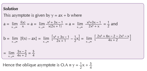
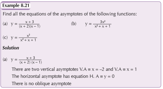
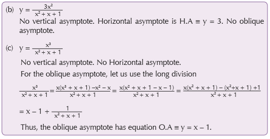
Note: For the rational functions;
- There is the oblique asymptote if the degree of the numerator is one greater than the degree of the denominator. An alternative way to find the equation of the oblique asymptote is to use a long division. There the equation is simply the quotient.
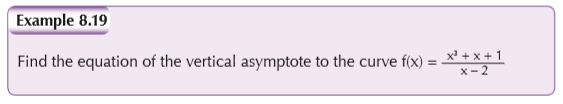
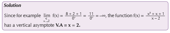
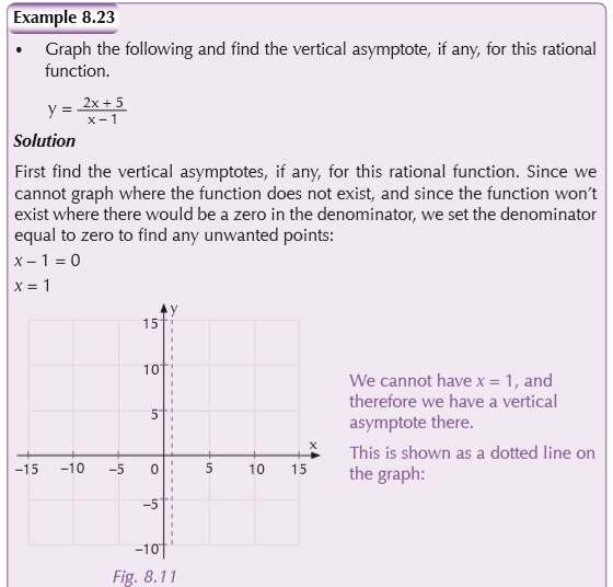
- The vertical asymptote, are found to be the values that make the denominator zero
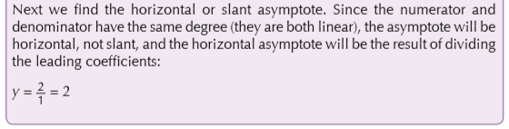
- For the horizontal asymptote, if the degree of the numerator is less than the degree of the denominator, then H.A ≡ y = 0. If the degree of the numerator is or equal to the degree of the denominator, then H.A ≡ y =

- The horizontal asymptote is the special case of the oblique asymptote.
Graphing asymptotes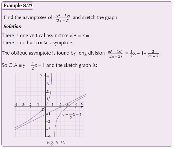
To graph a rational function, you find the asymptotes and the intercepts, plot a few points, and then sketch in the graph.


UNIT 9 : Differentiation of polynomials, rational and irrational functions, and their applications
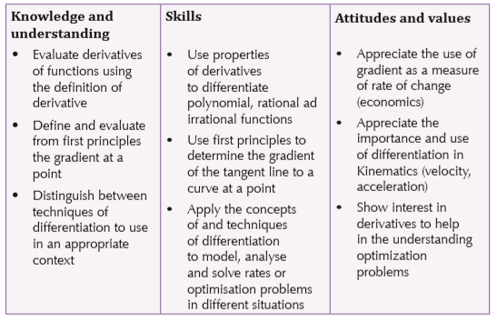
Key unit competence
Use the gradient of a straight line as a measure of rate of change and apply this to line tangents and normals to curves in various contexts. Use the concepts of differentiation to solve and interpret related rates and optimization problems in various contexts.
Learning objectives
9.1 Concepts of derivative of a function
Definition
Mental task
You have learnt about gradients. What is the gradient of a line? How is it obtained?
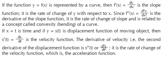
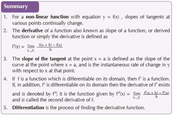
For a non-linear function with equation y = f(x), slopes of tangents at various points continually change.
The gradient of a curve at a point depends on the position of the point on the curve and is defined to be the gradient of the tangent to the curve at that point.
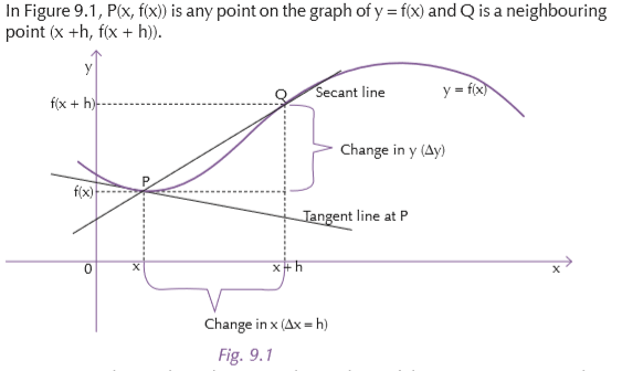
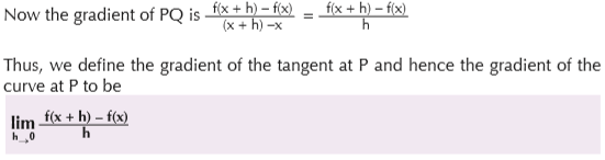
As Q approaches P along the curve, the gradient of the secant PQ approaches the gradient of the tangent at P. The gradient of the tangent at P is thus defined to be the limit of the gradient of the secant PQ as Q approaches P along the curve. i.e., as h → 0.
Derivative of a function
Activity 9.1
In groups of five, carry out research to find out the meaning of the term derivative in mathematics. Present your findings to the rest of the class.
How do we get the slope (gradient) at a point?
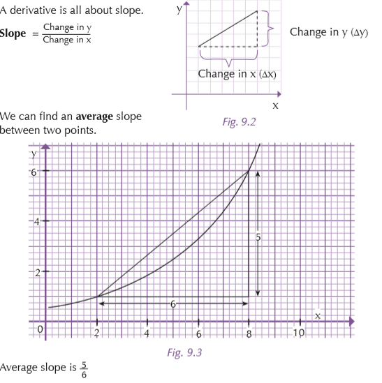
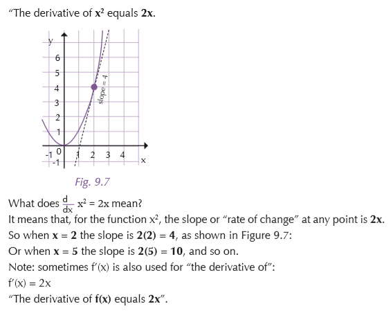
The derivative of a function y = f(x) at the point (x, f(x)) equals the slope of the tangent line to the graph at that point.
Let us illustrate this concept graphically.
Let f be a real-valued function and P (x, f(x)) be a point on the graph of this function. Let there be another point Q in the neighbourhood of P.
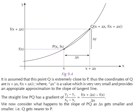
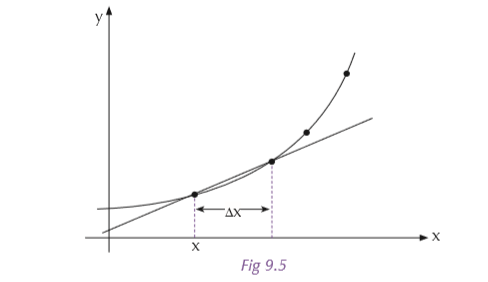
As the value of ∆x gets smaller, the two points get closer and the slope of PQ approaches that of the tangent line to the curve at P. As this happens the gradient of PQ will get closer to the slope of the tangent at P.
If we take this to the limit, as ∆x approaches 0, we will find the slope of the tangent at P and hence the gradient of the curve at P.

Activity 9.2
Work out the following in groups.
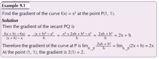
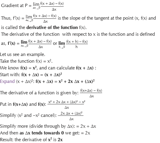
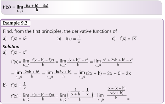
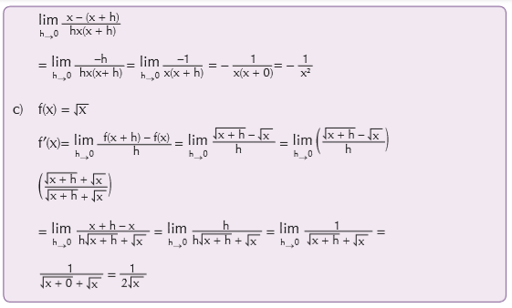
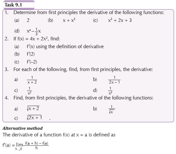
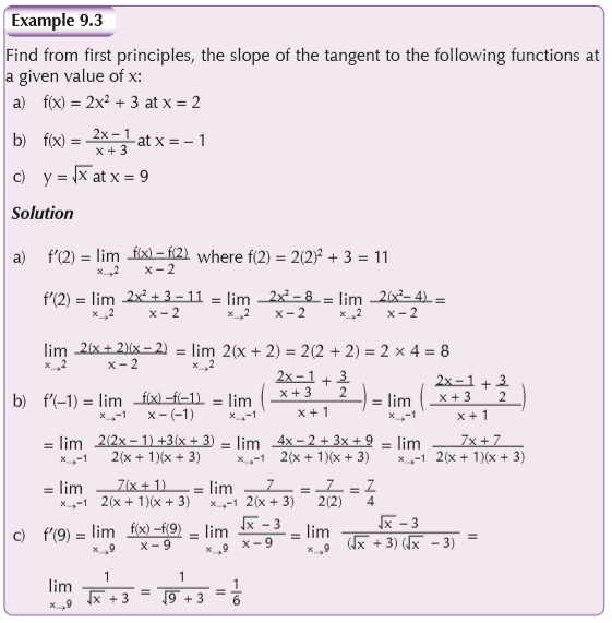
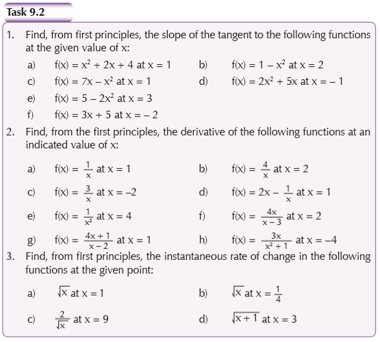
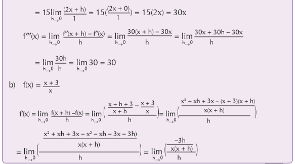
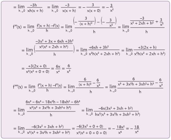
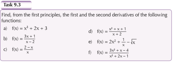
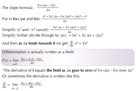
Differentiation from first principles
Finding the slope using the limit method is said to be using first principles, that is
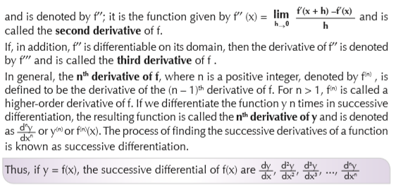
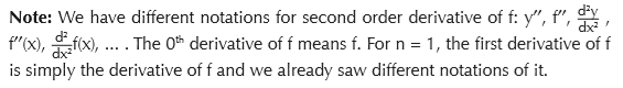
Higher order derivatives
If f is a function which is differentiable on its domain, then f′ is a derivative function. If, in addition, f′ is differentiable on its domain, then the derivative of f′ exists

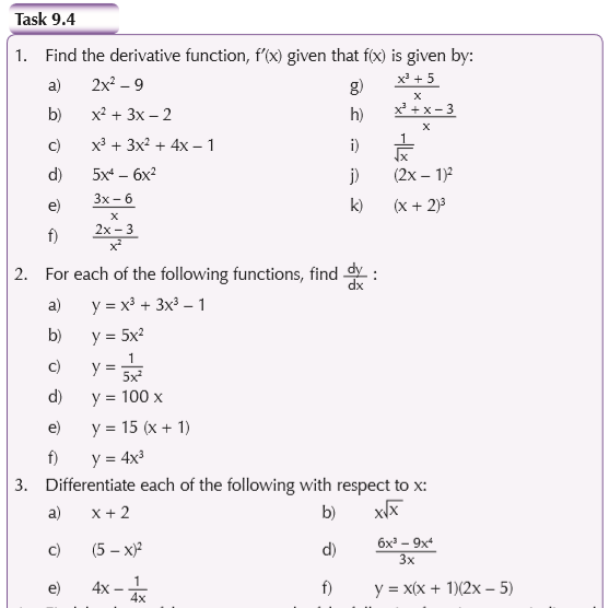
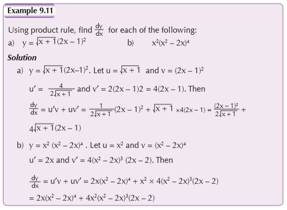
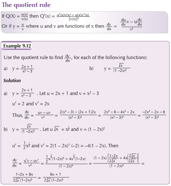
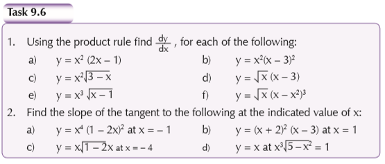
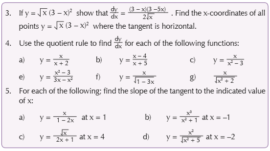
9.2 Rules of differentiation
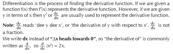

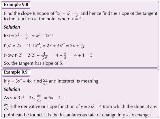
The process of finding a derivative is called “differentiation”.
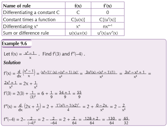
Below is the table containing basic rules which can be used to differentiate more complicated functions without using the differentiation from the first principles.
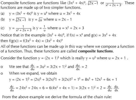
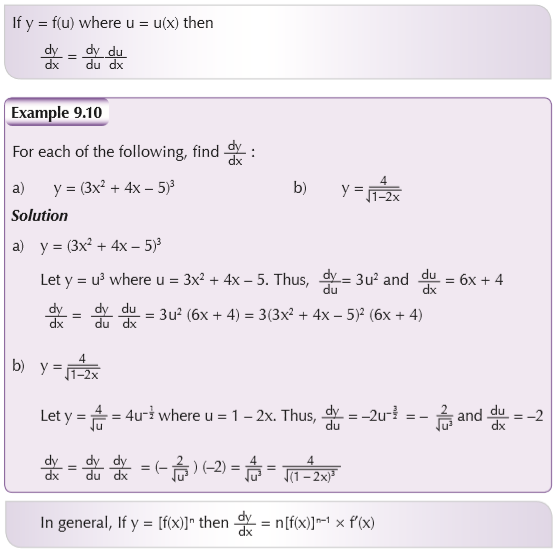
The chain rule
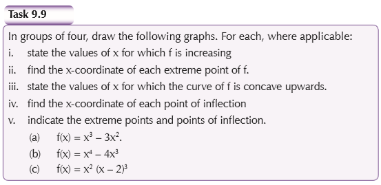
9.3 Applications of differentiation
Geometric interpretation of derivatives
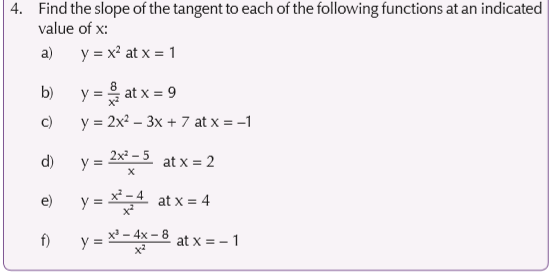
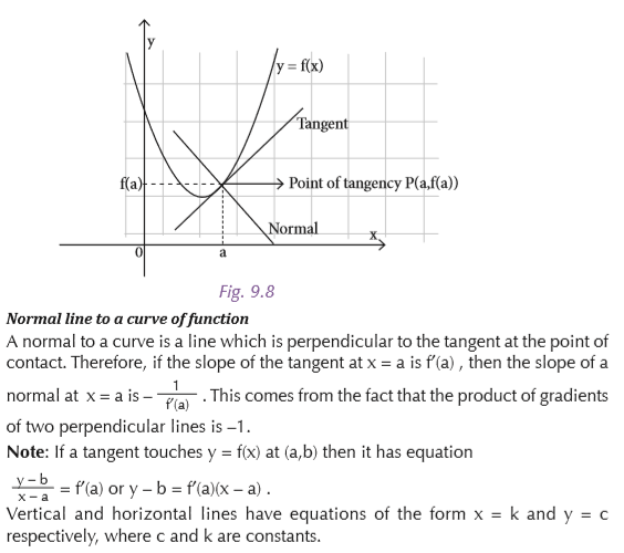
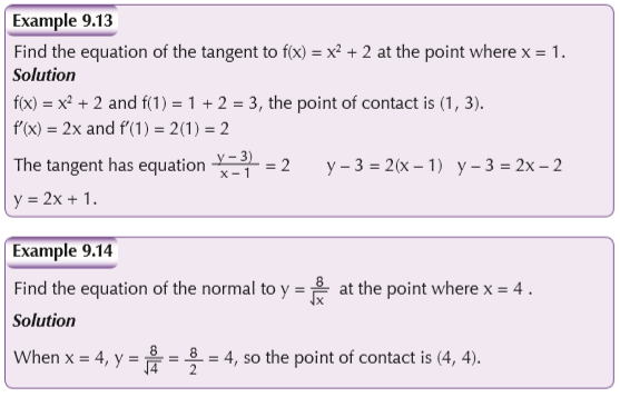
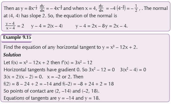
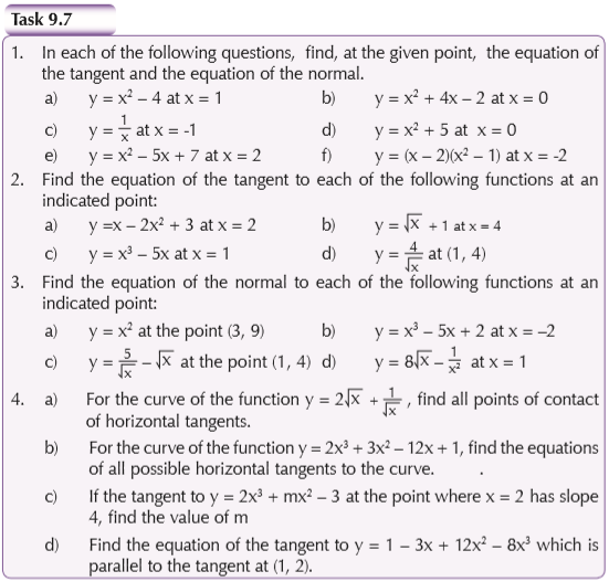
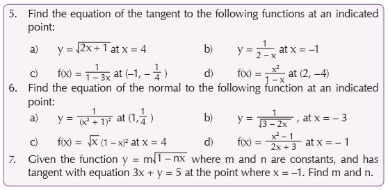
Equations of tangent and normal to a curve
Tangent line to a curve of function
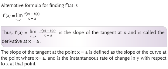
Consider a curve y = f(x) . If P is the point with x-coordinate a, then the slope of the tangent at this point is f′(a) .The equation of the tangent is by equating slopes and is

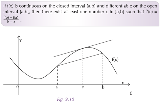
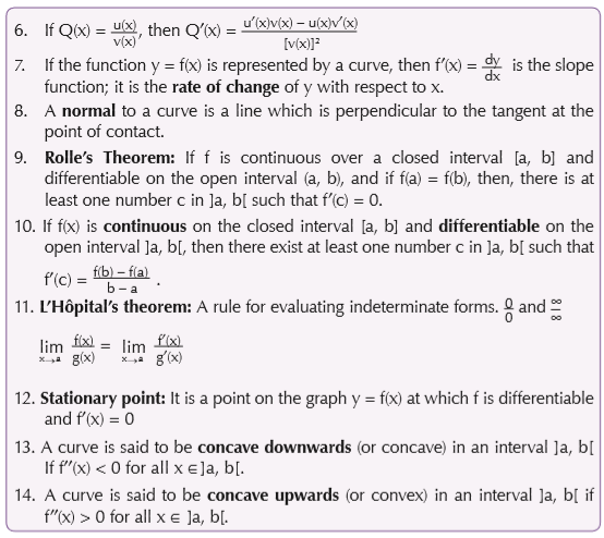
Mean value theorems
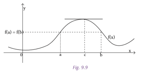
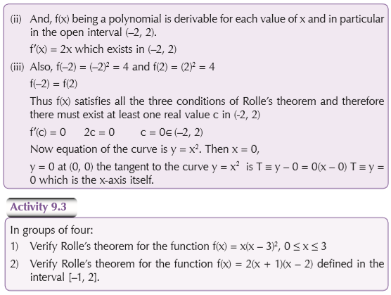
Rolle’s theorem
If f is continuous over a closed interval [a,b] and differentiable on the open interval (a,b), and if f(a) = f(b), then, there is at least one number c in ]a,b[ such that f′(c)=0.

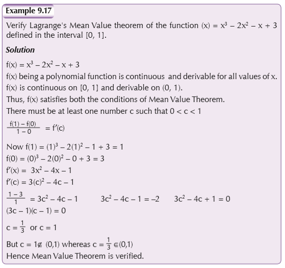
Lagrange’s mean value theorem
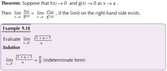
L’Hôpital theorem
This is a rule for evaluating indeterminate forms. One of the forms of the rule is the following:
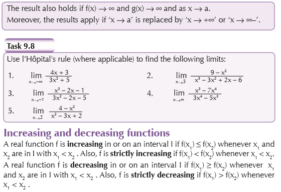

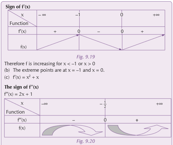
Meaning of the sign of the derivative
If we recall that the derivative of a function yields the slope of the tangent to the curve of the function. It appears that a function is increasing at a point where the derivative is positive and decreasing where the derivative is negative.
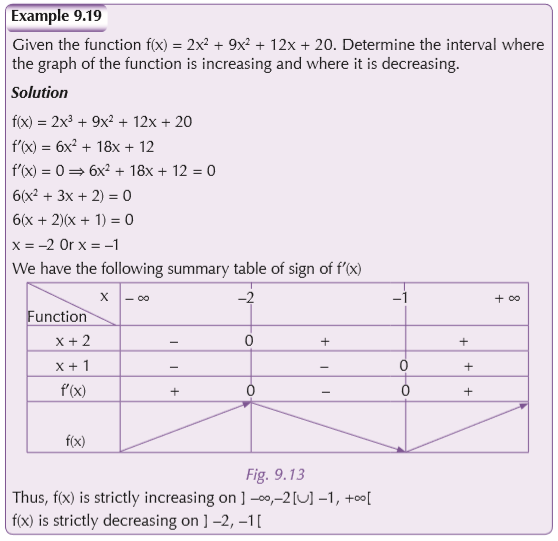
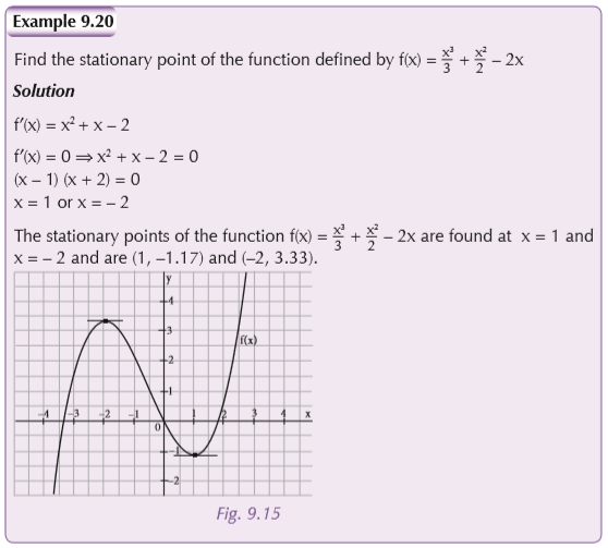
Stationary point
This is a point on the graph y = f(x) at which f is differentiable and f′(x) = 0. The term is also used for the number c such that f′(c) . The corresponding value f(c) is a stationary value. A stationary point c can be classified as one of the following, depending on the behaviour of f in the neighbourhood of c:
(i) A local maximum, if f′(x) > 0 to the left of c and f′(x) < 0 to the right of c,
(ii) A local minimum, if f′(x) < 0 to the left of c and f′(c) > 0to the right of c,
(iii) Neither local maximum nor minimum.
Note: Maximum and minimum values are termed as extreme values.

The points a, b and c are stationary points.
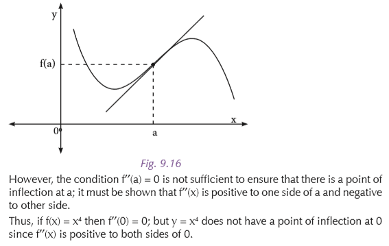
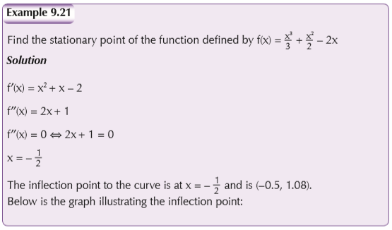
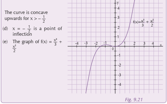
Point of inflection
A point of inflection is a point on a graph y = f(x) at which the concavity changes. If f′ is continuous at a, then for y = f(x) to have a point of inflection at a it is necessary that f′′(a) =0, and so this is the usual method of finding possible points of inflection.
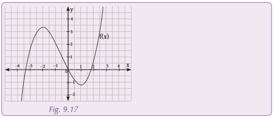
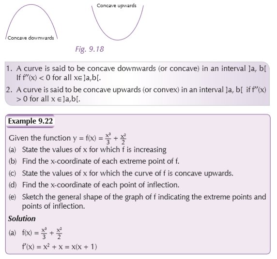
Concavity
At a point of graph y = f(x), it may be possible to specify the concavity by describing the curve as either concave up or concave down at that point, as follows:
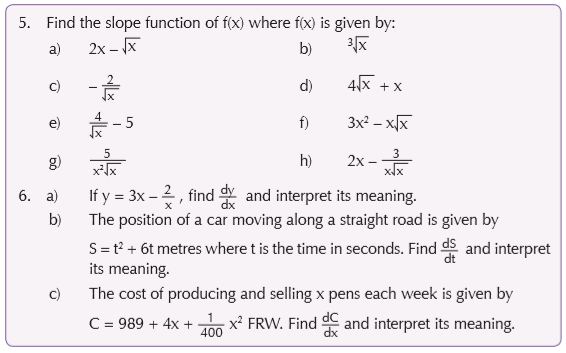
Rate of change problems
Mental task
We can use differentiation to help us solve many rate of change problems. Can you mention any such problems?
Gradient as a measure of rate of change
Kinematic meaning of derivatives
Motion of a body on a straight line
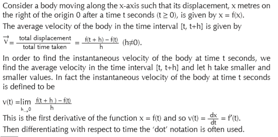
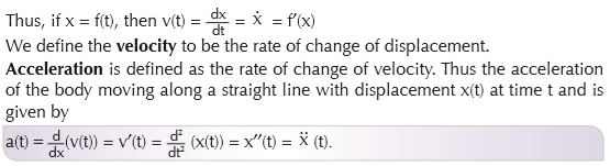
Velocity is a vector quantity and so the direction is critical. If the body is moving towards the right (the positive direction of the x-axis), its velocity is positive and if it is moving towards the left, its velocity is negative. Therefore, the body changes motion when velocity changes sign. A sign diagram of the velocity provides a deal with information regarding the motion of the body.
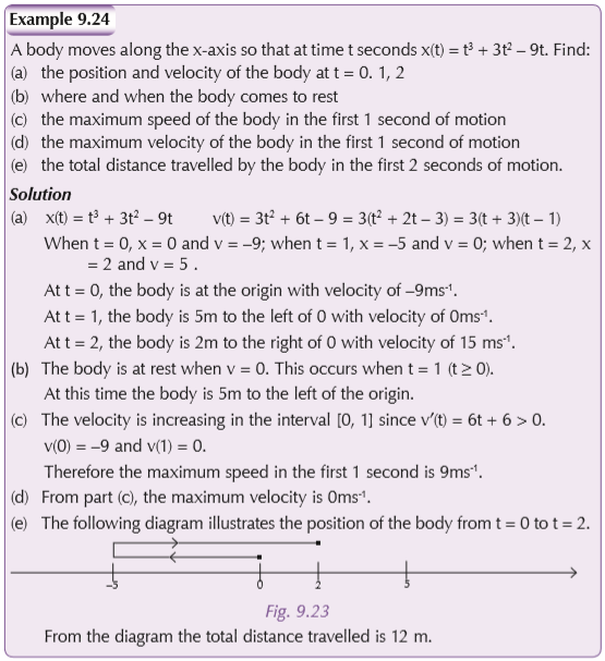

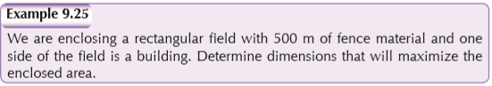
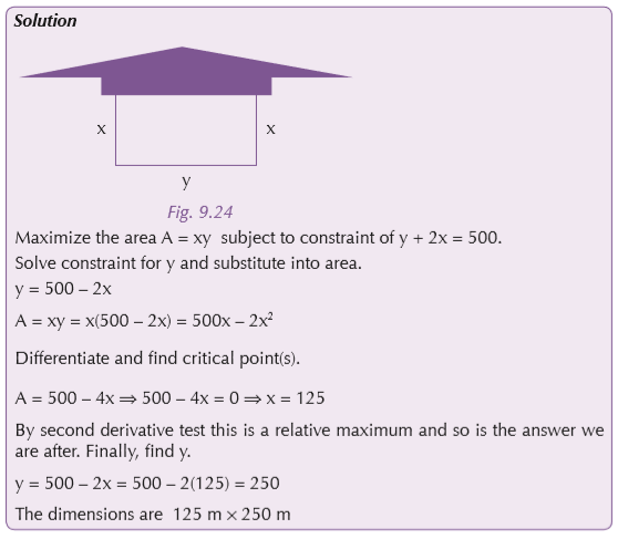
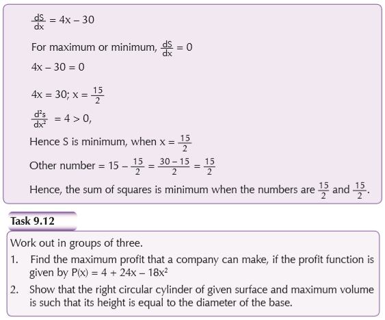
Optimization problems
Activity 9.4
Carry out research on the meaning of optimization. Where is optimization applied?
Mathematical optimization is the selection of a best element (with regard to some criteria) from some set of available alternatives.
In the simplest case, an optimization problem consists of maximizing or minimizing a real function by systematically choosing input values from within an allowed set and computing the value of the function.
UNIT 10 : Vector space of real numbers
Key unit competence
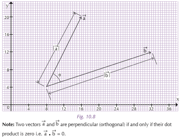
Determine the magnitude and angle between two vectors and to be able to plot these vectors. Also, be able to point out the dot product of two vectors.
Learning objectives
10.1 Vector spaces lR2
Definitions and operations on vectors
In Senior 2, we were introduced to vector and scalar quantities.
Task 10.1
1. Define a vector.
2. Differentiate between a vector and a scalar quantity.
3. Use diagrams to illustrate equal vectors.
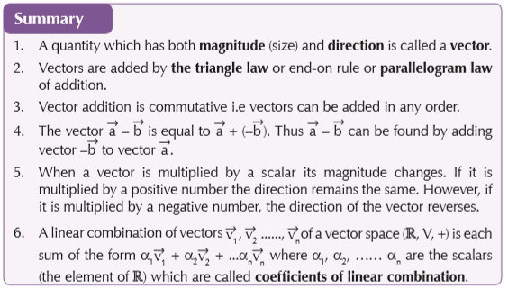
A quantity which has both magnitude and direction is called a vector. It is usually represented by a directed line segment. In our daily life, we deal with two mathematical quantities:
(a) one which has a defined magnitude but for which direction has no meaning (example: length of a piece of wire).
In physics, length, mass and speed have magnitude but no direction. Such quantities are defined as scalars.
(b) the other for which direction is of fundamental significance. Quantities such as force and wind velocity depend very much on the direction in which they act. These are vector quantities.
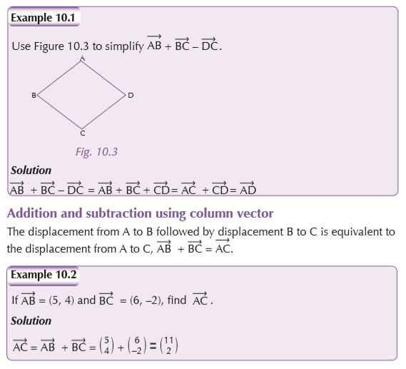
Addition of vectors
Vectors are added by the triangle law or end-on rule or parallelogram law of addition.
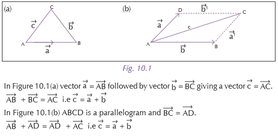
The parallelogram law
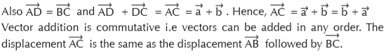
Vector subtraction
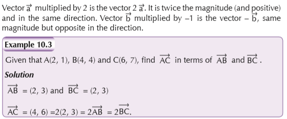
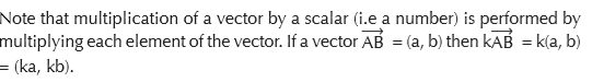
Multiplication of a vector by a scalar
When a vector is multiplied by a scalar (a number) its magnitude changes. If it is multiplied by a positive number the direction remains the same.
However, if it is multiplied by a negative number, the direction of the vector reverses.
10.2 Vector spaces of plane vectors ( lR, V, +)
The definition of vector space denoted by V needs the arbitrary fields F = whose elements are called scalars.
Definitions and operations
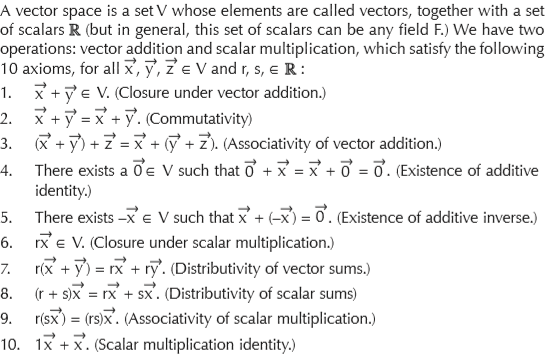
Properties of vectors
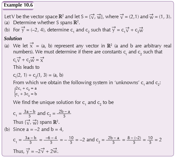
Linear combination of vectors
Spanning vectors
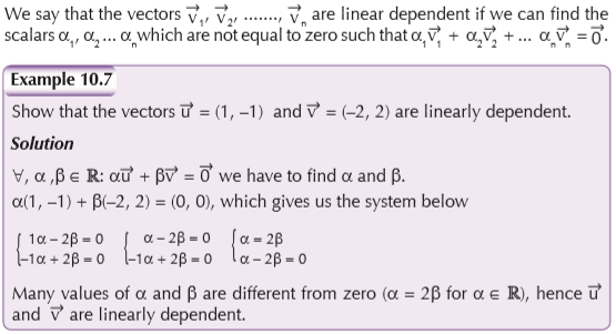
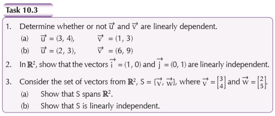
Linear dependent vectors
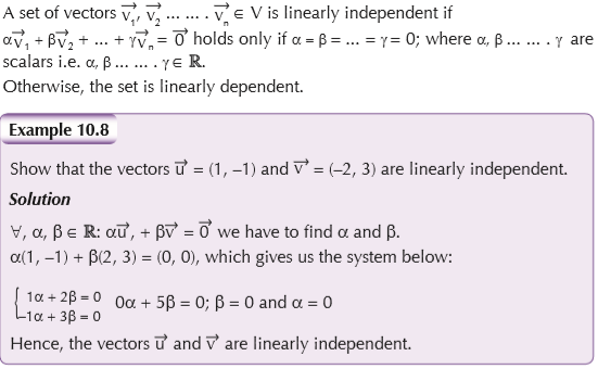
Linear independent vectors
Basis and dimension of a vector space
Dimension of vector space
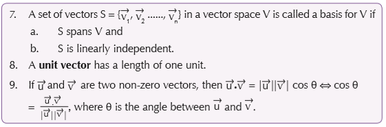
The dimension of a non-zero vector space V is the number of vectors in a basis for V. Often we write Dim (V) for the dimension of V.
For lRn , one basis is the standard basis, and it has n vectors. Thus, the dimension of n is lRn.
10.3 Euclidian vector space
Activity 10.1
In groups, carry out research to determine the similarities between vector spaces and Euclidian spaces.
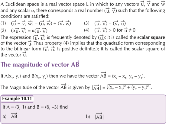
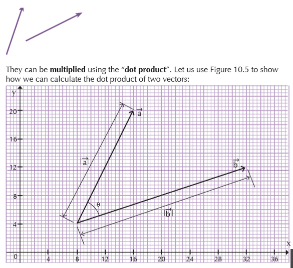
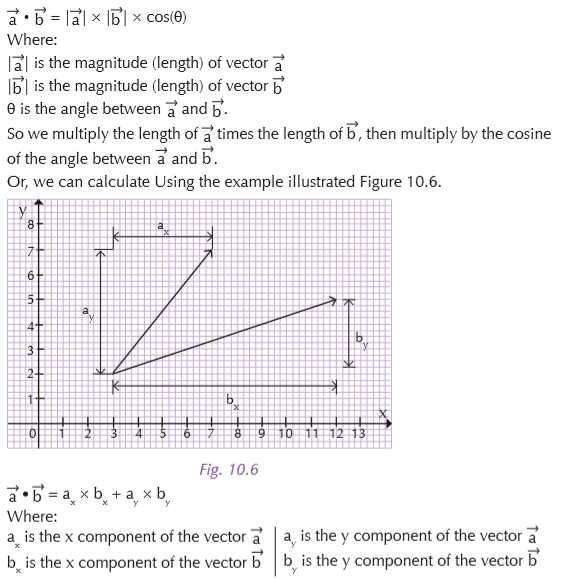
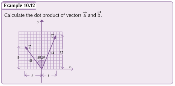
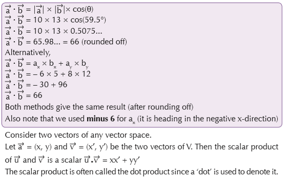
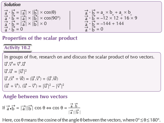
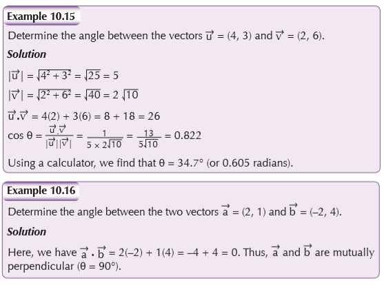
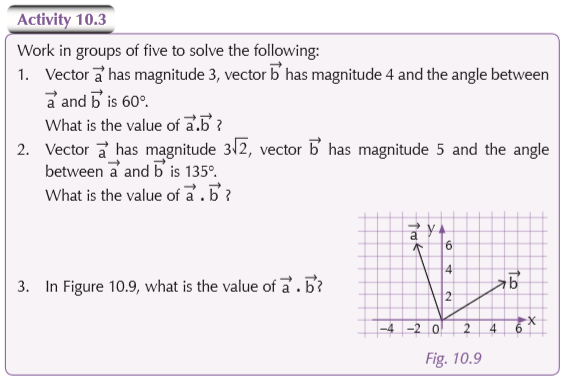
Dot product and properties
These are vectors:


UNIT 11 : Concepts and operations on linear transformations in 2D
Key unit competence
Determine whether a transformation of IR2 is linear or not. Perform operations on linear transformations.
Learning objectives

11.1 Linear transformation in 2D
Activity 11.1
What is transformation as is used in mathematics? What is linear transformation? Research on the different types of 2D linear transformations. Discuss your findings with the rest of the class.
Definitions
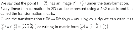
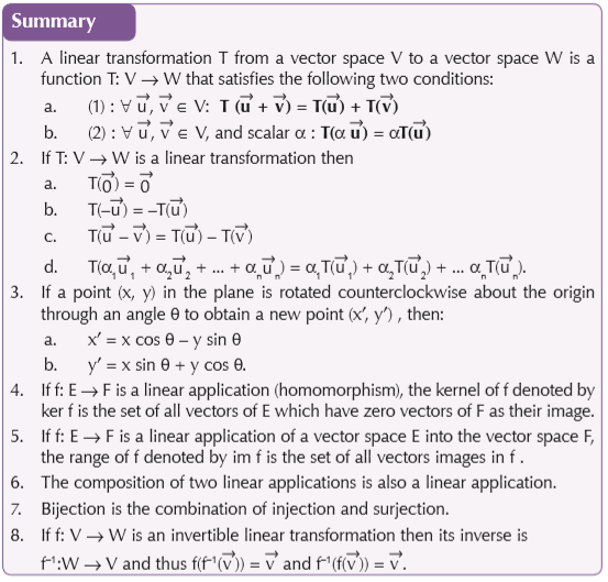
A linear transformation T from a vector space V to a vector space W is a function
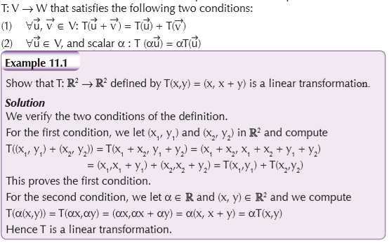
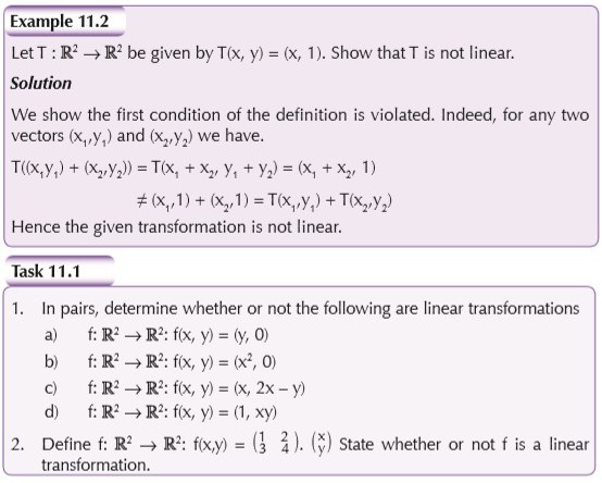
Properties of linear transformations

11.2 Geometric transformations in 2D
Activity 11.2
Research on the meaning of geometric transformations. How many types can you list, with examples? Discuss your findings in class.
A geometric transformation is an operation that modifies the position, size, shape and orientation of the geometric object with respect to its current state and position.
Reflection
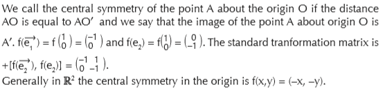
Generally, a reflection is a transformation representing a flip of a figure. Figures may be reflected in a point, a line, or a plane. When reflecting a figure in a line or in a point, the image is congruent to the preimage.
A reflection maps every point of a figure to an image across a line of symmetry using a reflection matrix.
Use the following rule to find the reflected image across a line of symmetry using a reflection matrix.
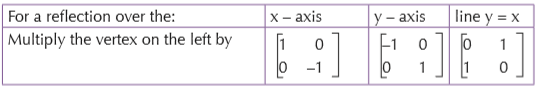
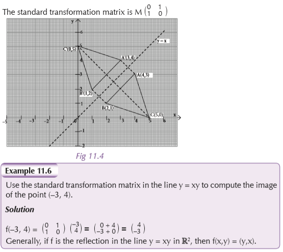
Reflection (symmetry) about x-axis
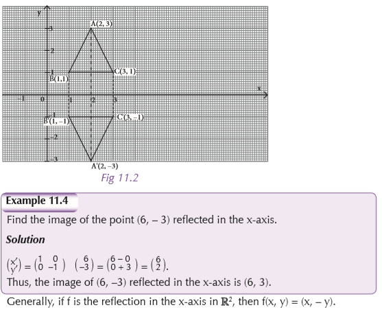
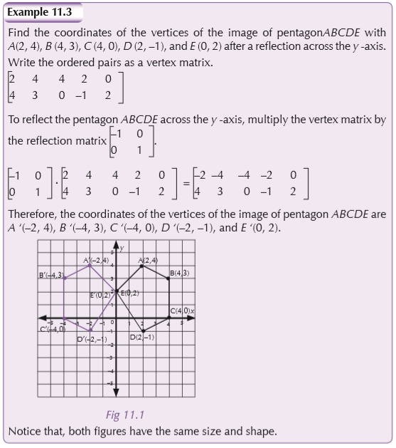
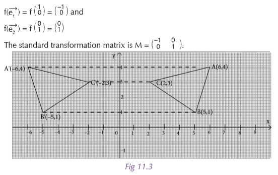
Reflection (symmetry) about y-axis
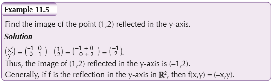
Reflection (symmetry) about the line y = x
Central symmetry
Identical transformation

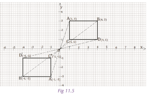
Rotation
A rotation is a transformation in a plane that turns every point of a preimage through a specified angle and direction about a fixed point. The fixed point is called the center of rotation. The amount of rotation is called the angle of rotation and it is measured in degrees.
A rotation maps every point of a preimage to an image rotated about a centre point, usually the origin, using a rotation matrix.
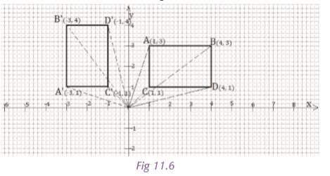
Use the following rules to rotate the figure for a specified rotation. To rotate
counterclockwise about the origin, multiply the vertex matrix by the given matrix.
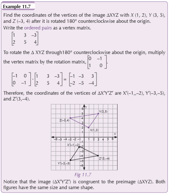
Rotation about origin with angle θ
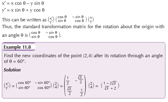
If a point (x, y) in the plane is rotated counterclockwise about the origin through an angle θ to obtain a new point (x′, y′), then
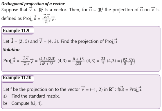
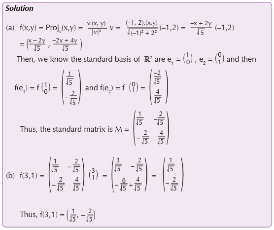
Orthogonal and orthonormal transformation
A set of vectors is said to be orthogonal if all pairs of vectors in the set are perpendicular.
A set of vectors is said to be orthonormal if it is an orthogonal set and all the vectors have unit length.
11.3 Kernel and range
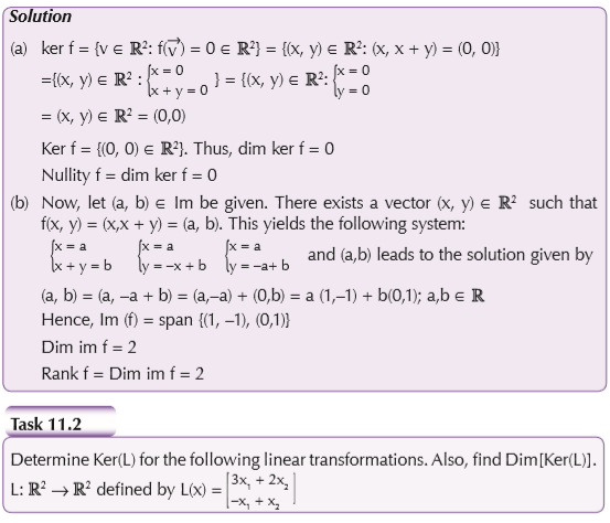
Kernel and image of linear transformation
The kernel of a linear transformation
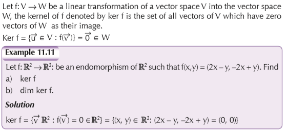
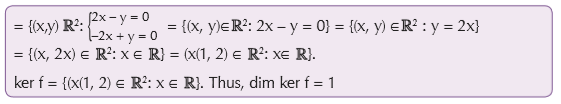
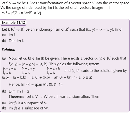
The range (image) of a linear transformation
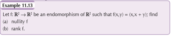
Nullity and rank
The dimension of the kernel is called the nullity of f (denoted nullity f) and the dimension of the range of f is called the rank of f (denoted rank f).
11.4 Operations of linear transformation
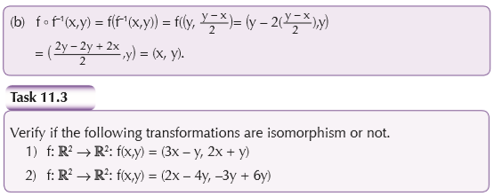
Activity 11.3
In pairs, carry out research to find out what is linear transformation. How do we sum up two linear transformations and how do we compose them?
Addition
f: V → W and g: V → W
f + g = V → W: (f + g)( a ) = f( a ) + g( a ). The sum of two linear transformations is a linear transformation.
Composition of two linear transformations
Let f: V → W and g: V → W then the composite of f and g, (g f) is a linear transformation
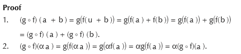
Therefore, the composition of two linear transformations is also a linear transformation.
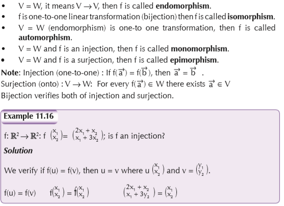
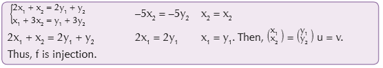
One-to-one linear transformation
A linear transformation f is said to be a one-to one if for each element in the range there is a unique element in the domain which maps to it.
Onto linear transformation
A linear transformation f is said to be onto if for every element in the range space there exists an element in the domain that maps to it.
Isomorphism
The word isomorphism comes from the Greek word which means ‘equal shape’. An isomorphism is a linear transformation which is both one-to-one and onto.
If two vector spaces V and W have the same basic structures, then there is an isomorphism between them. Dim V = Dim W.
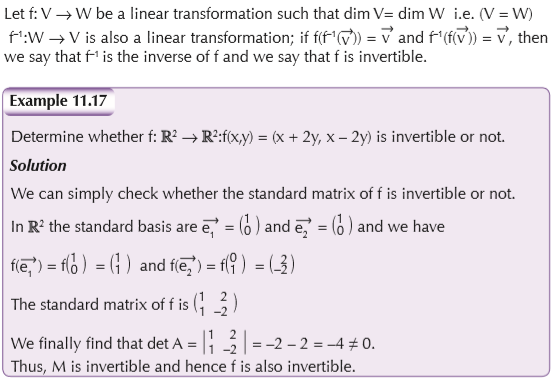
Note: A linear transformation has an inverse if and only if it is an isomorphism.
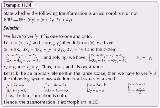
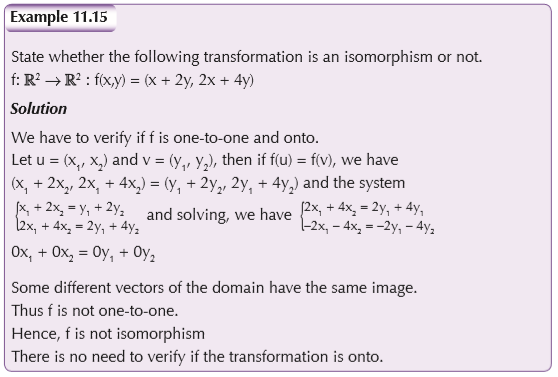
Note: A transformation fails to be isomorphism if it fails to be either one-to-one or onto.
Remark: For the linear application f: V → W when
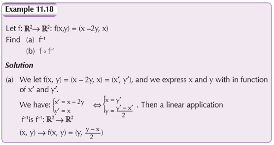
Inverse of linear transformation
UNIT 12 : Matrices and determinants of order 2
Key unit competence
Use matrices and determinants of order 2 to solve systems of linear equations and to define transformations of 2D.
Learning objectives
12.1 Introduction
Activity 12.1
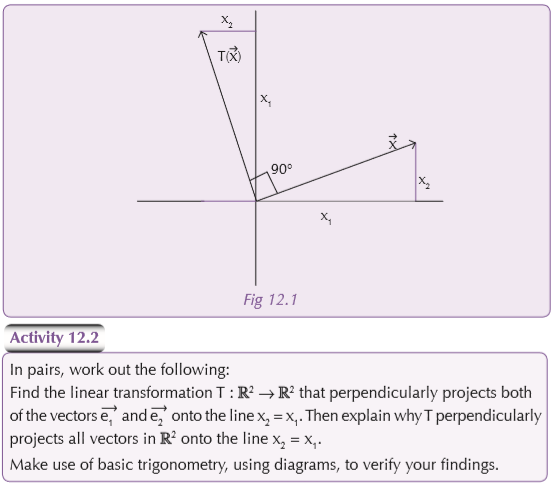
In pairs, carry out research to find out the meaning of the term matrix. What is the plural of matrix? Where and when can we make use of a matrix?
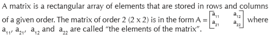
A matrix is an ordered set of numbers listed in rectangular form.
Order of a matrix
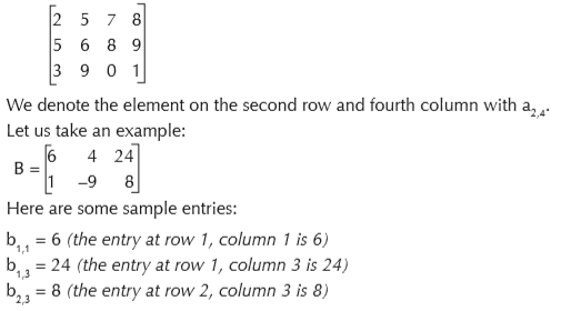
The number of rows and columns that a matrix has is called its order or its dimension. By convention, rows are listed first; and columns, second. Thus, we would say that the order (or dimension) of the matrix below is 3 x 4, meaning that it has 3 rows and 4 columns.
Square matrix
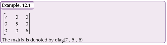
Diagonal matrix
A diagonal matrix is a square matrix with all non-diagonal elements 0. The diagonal matrix is completely defined by the diagonal elements.
Row matrix
A matrix with one row is called a row matrix.
[2 5 –1 5]Column matrix
A matrix with one column is called a column matrix.

We talk about one matrix, or several matrices. There are many things we can do with them.
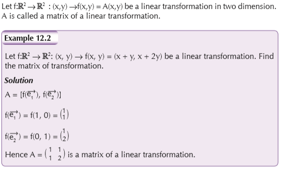
12.2 Matrix of a linear transformation
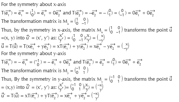
12.3 Matrix of geometric transformation
Symmetric about x-axis and y-axis
Rotation

12.4 Operations on matrices
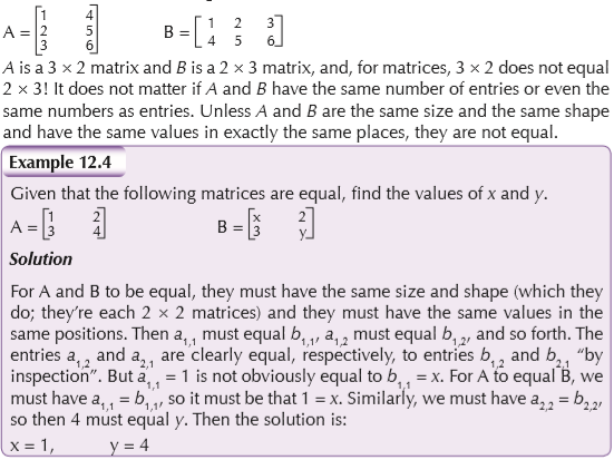
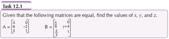
Equality of matrices
Activity 12.3
Carry out research to find out the meaning of equal matrices. Discuss in class using examples.
For two matrices to be equal, they must be of the same size and have all the same entries in the same places. For instance, suppose you have the following two matrices:
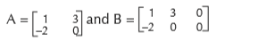
These matrices cannot be the same, since they are not of the same size. If A and B are the following two matrices:
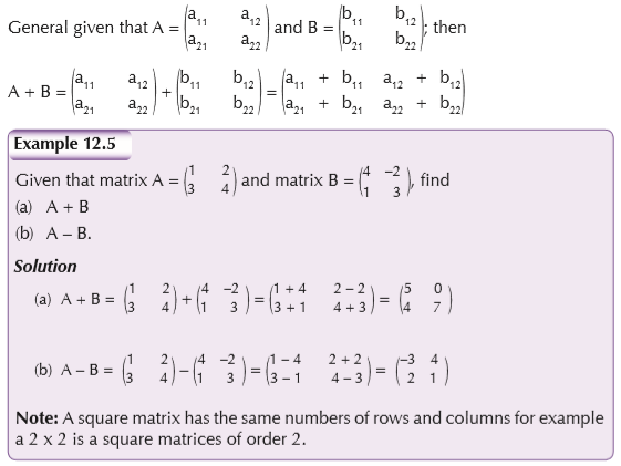
Addition and subtraction of matrices
Addition and subtraction of matrices is only possible for matrices of the same order.
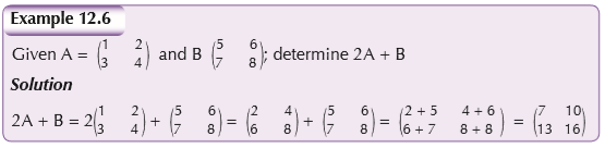
Addition
To add two matrices: add the numbers in the matching positions:

The two matrices must be of the same size, i.e. the rows must match in size, and the columns must match in size.
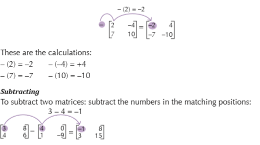
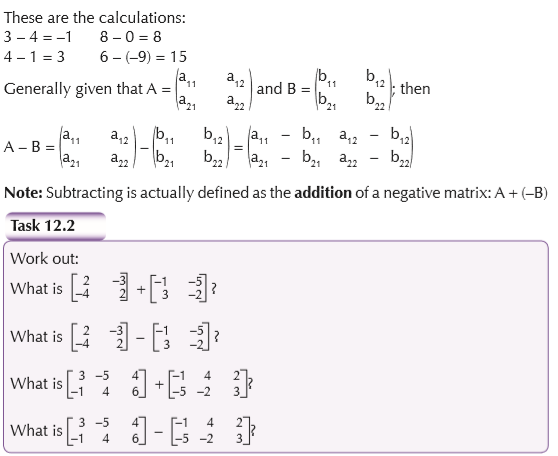
Subtraction
Negative
The negative of a matrix is also simple:
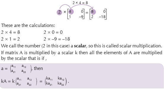
Multiplication of a matrix by a scalar
To multiply a matrix by a single number is easy:
Identity matrix

Multiplication of matrices
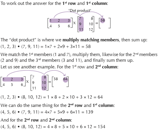
Two matrices can be multiplied if and only if the number of columns of the first matrix is equal to the number of rows of the second matrix. Such matrices are said to be compatible to multiplication.
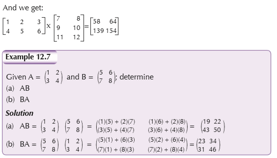
To multiply a matrix by another matrix we need to use the dot product of rows and columns.
Let us see using an example:
Transpose of a matrix
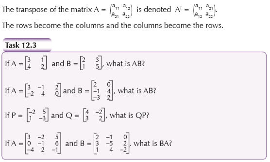
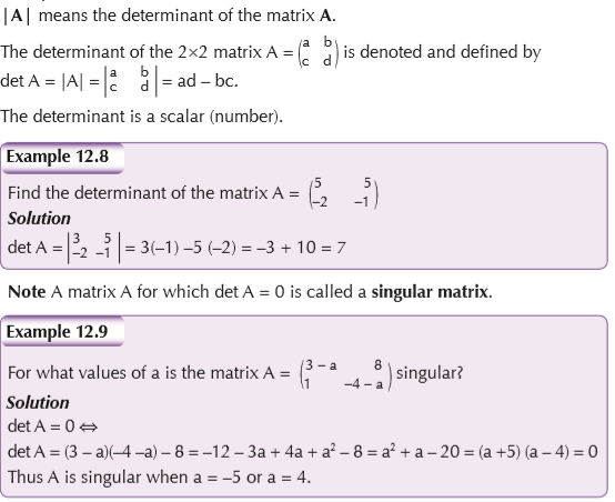
12.5 Determinant of a matrix of order 2
Activity 12.4
In pairs, find out the meaning of the term determinant as used in the case of matrices. Why do we need determinants? What is the symbol for determinant?
The determinant of a matrix is a special number that can be calculated from a square matrix. The symbol for determinant is two vertical lines either side. For example,
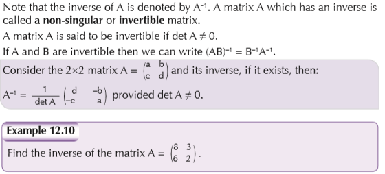
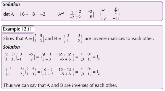
Inverse of matrices
If A is a square matrix then a matrix B such that AB = BA = I2 is called an inverse of the matrix A.
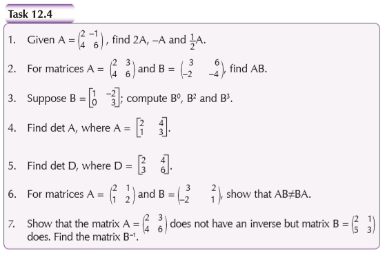
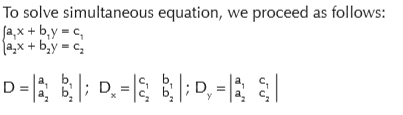
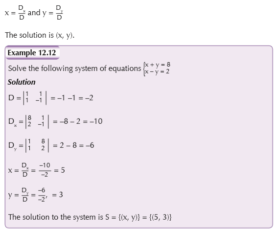
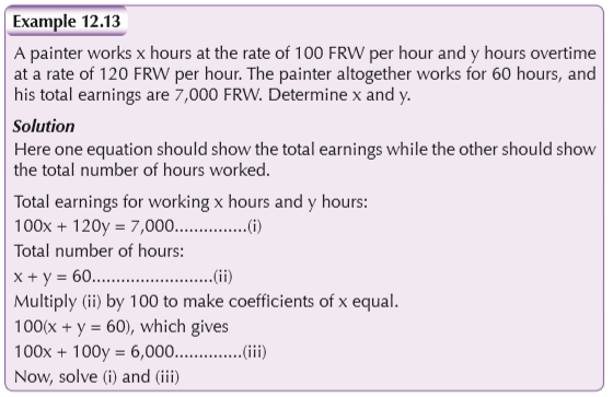
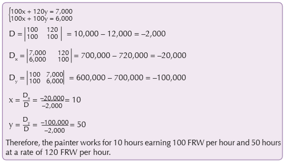
Application of determinants
Cramer’s method
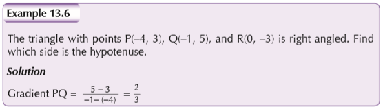
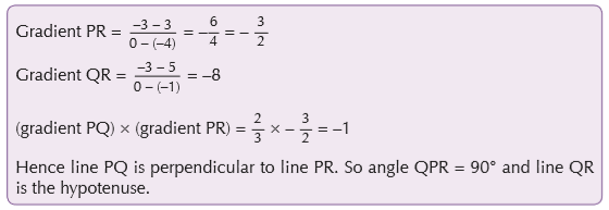
UNIT 13 : Points, straight lines and circles in 2D
Key unit competence
Determine algebraic representations of lines, straight lines and circles in 2D.
Learning objectives
13.1 Points in 2D
Activity 13.1
What is a point?
In Junior Secondary, we studied points on a Cartesian plane. How do we define the coordinate of a point in 2D? Discuss in groups and present your findings to the rest of the class
A point is an exact position or location on a plane surface. It is important to understand that a point is not a thing, but a place. We indicate the position of a point by placing a dot with a pencil. In coordinate geometry, points are located on the plane using their coordinates - two numbers that show where the point is positioned with respect to two number line “axes” at right angles to each other.
Cartesian coordinate of a point
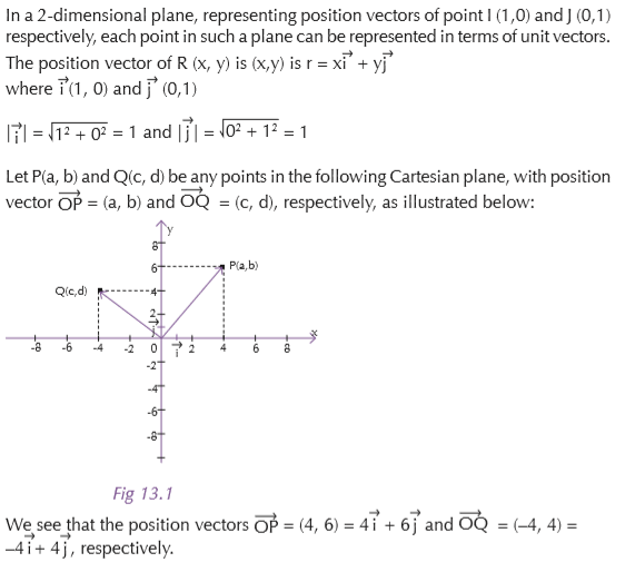
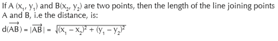
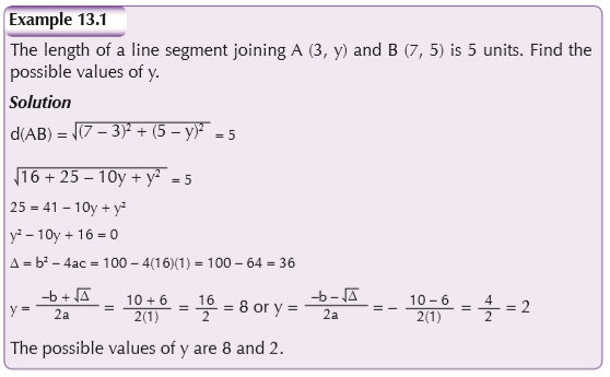
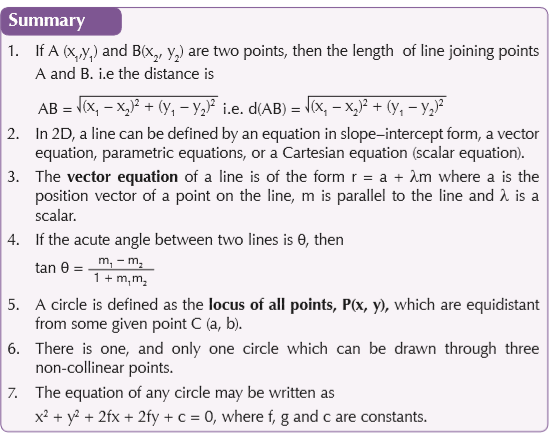
Distance between two points
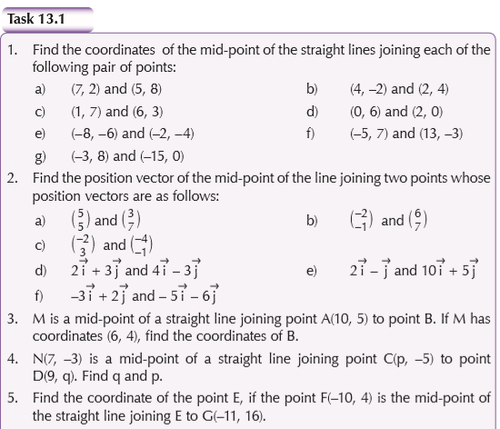
The mid-point of a line segment

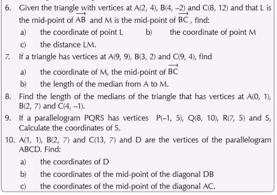
13.2 Lines in 2D
The equations of straight lines
A particular line is uniquely located in a plane if
• it has a known direction and passes through a known fixed point, or
• it passes though two known points.
Cartesian equation of a straight line
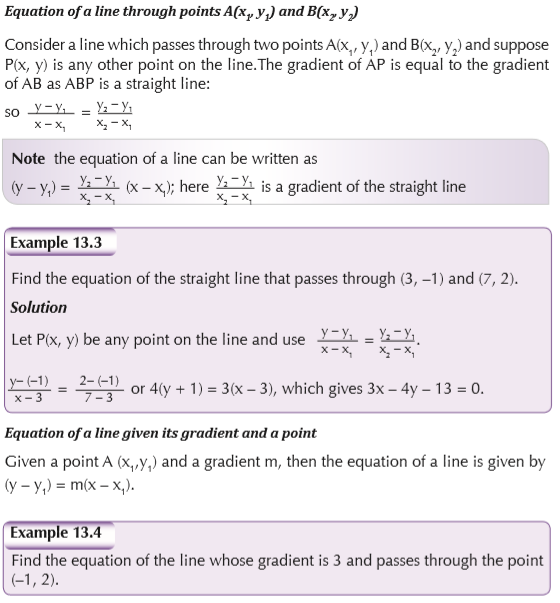
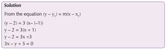
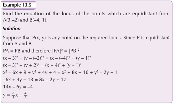
Equation of a line given a law
We can find the equation of the locus by considering a point P(x, y) on the locus and using the law to derive an equation in x and y. This will be the equation of the locus.
Parallel and perpendicular lines
If two lines are parallel, they have equal gradients
If two lines are perpendicular, the product of their gradients is –1.

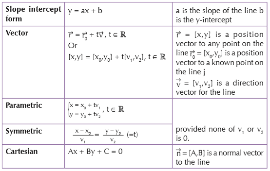
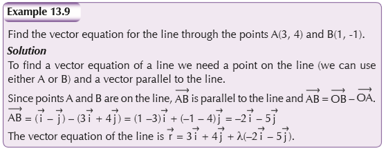
Vector, parametric, scalar and Cartesian equations of the line
In 2D, a line can be defined by an equation in slope–intercept form, a vector equation, parametric equations, or a Cartesian equation (scalar equation).

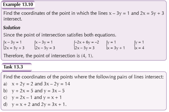
Intersection of lines with equations in Cartesian form
Any point on a line has coordinates which will satisfy the equation of that line. In order to find the point in which two lines intersect we have to find a point with coordinates which satisfy both equations. This is equivalent, from an algebraic point of view, to solving the equations of the lines simultaneously.
The intersection of two lines with equations given in vector form
In order to find the point of intersection of two lines whose equations are given in vector form each equation must have a separate parameter. The method as illustrated in the following example:

13.3 Points and lines
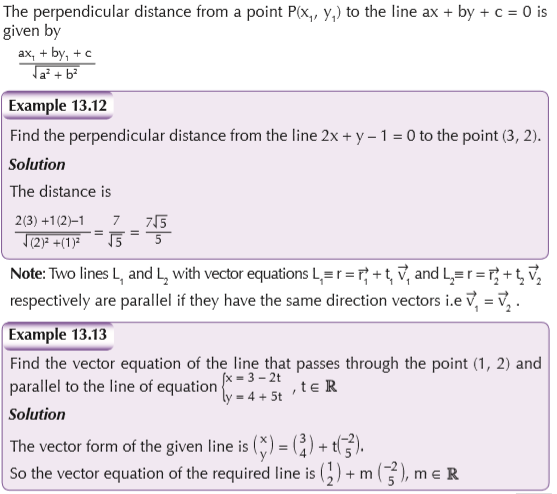
Distance of a point from a line
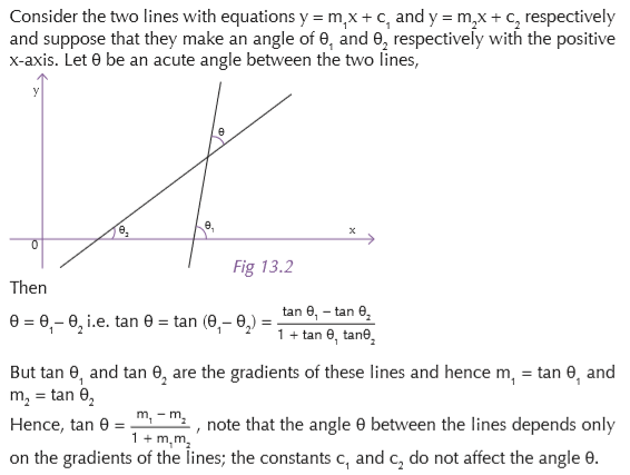
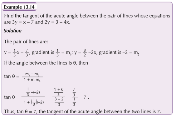
Angle between two straight lines
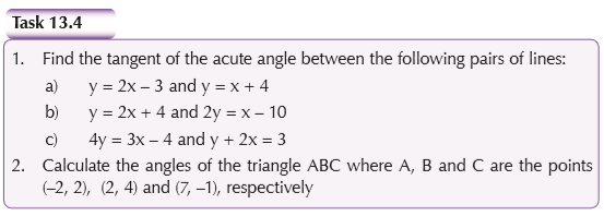
13.4 The circle
Mental task
What is a circle? What are the main parts of a circle that you can recall? Why are they significant?
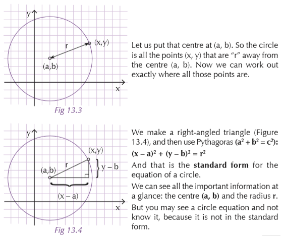
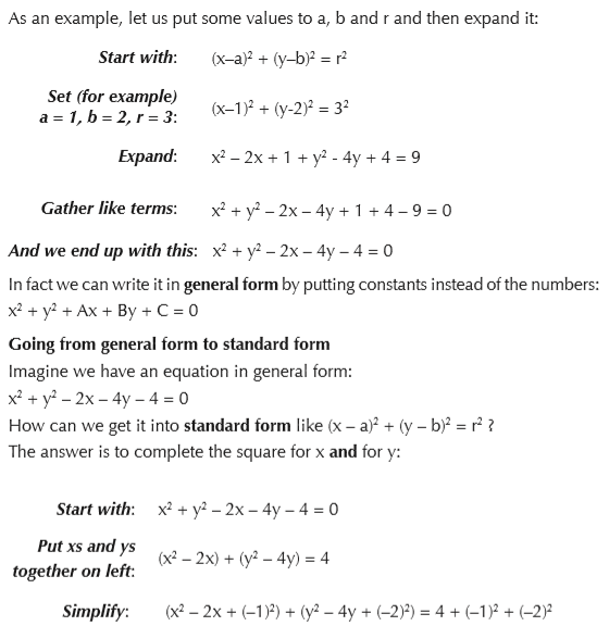
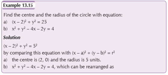
In fact the definition of a circle is: the set of all points on a plane that are at a fixed distance from a centre.

Unit circle
If we place the circle centre at (0,0) and set the radius to 1 we get:

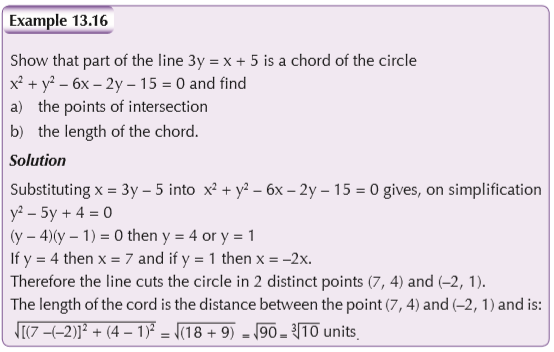
Intersecting a line and a circle
Consider a straight line y = mx + c and a circle (x – a)2 + (y – b)2 = r2.
There are three possible situations:
1. The line cuts the circle in two distinct places, i.e. part of the line is a chord of the circle.
2. The line touches the circle, i.e. the line is a tangent to the circle.
3. The line neither cuts nor touches the circle.
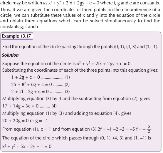
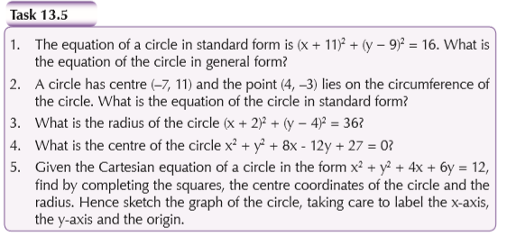
Circle through three given points
Three non-collinear points define a circle,
i.e. there is one, and only one circle which can be drawn through three non-collinear points. The equation of any
UNIT 14 : Measures of dispersion
Key unit competence
Extend understanding, analysis and interpretation of data arising from problems and questions in daily life to include the standard deviation.
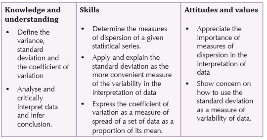
Learning objectives
14.1 Introduction
In Junior Secondary, you were introduced to statistics. You learnt about measures of central tendencies. In this unit, we shall learn about measures of dispersion.
Activity 14.1
Discuss in groups the meaning of measures of central tendencies. What are they? Where can we apply them?
Definitions
A measure of central tendency; also called average, is values about which the distribution of data is approximately balanced. There are three types of measure of central tendency namely the mean, the median and the mode.
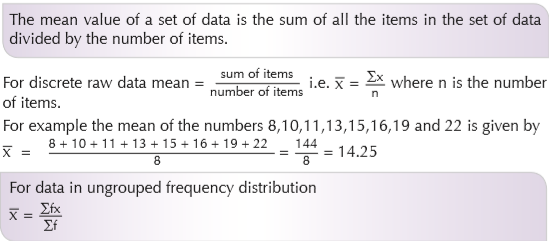
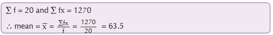
Mean: is the sum of data values divided by the number of values in the data.
Mode: is the value that occurs most often in the data.
Median: is the middle value when the data is arranged in order of magnitude.
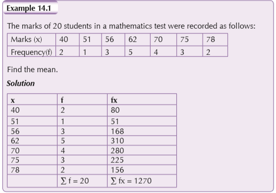
The mean
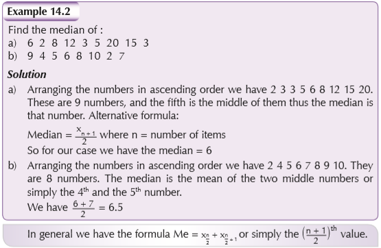
The median
The median of data is the middle value when all values are arranged in order of the size.
When the number of the items is odd then the median is the item in the middle. If and when the number of items is even, the median is the mean of the two numbers in the middle.
The mode
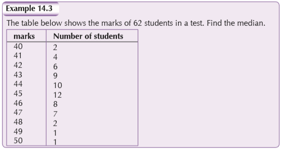
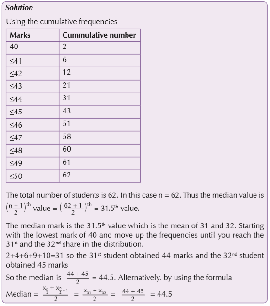
The mode of a set of data is the value of the higher frequency in the distribution of marks
In Example 14.3 the mode is 45 because it has the highest frequency, 12.
Grouped data
Grouped data is commonly used in continuous distribution data that takes any value in a given range is called continuous data.
Such data has values which are only approximations, such as height, weight, mass, time, age and temperature.
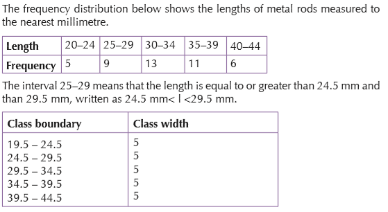
The mean of grouped data
In order to find the mean of the grouped data:
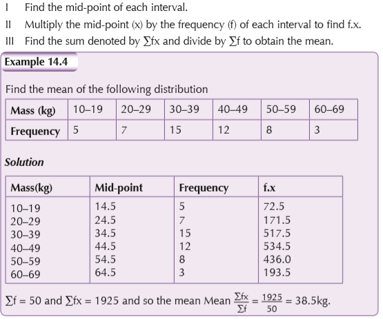
The mean from an assumed mean
When data is grouped in classes of equal width, we use the assumed mean in order to reduce the numerical size of the value of n.
Determine the mid-point of each class interval and the classes of the central value of x which is usually the modal value. This value is referred to as an assumed value or working mean.
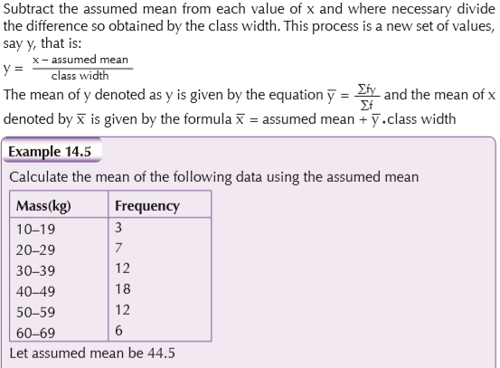
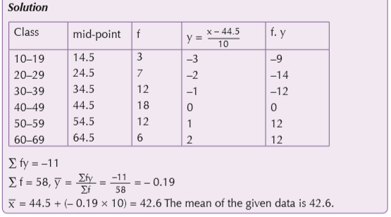
14.2 Measures of dispersion
Activity 14.2
In groups of three, research on the meaning and types of measures of dispersion. Why are they useful? Discuss your findings with the rest of the class.
A measure of dispersion is the degrees of spread of observation in data. The common measure of dispersion are range inter-quartiles, range and the standard deviation (the square root of the variance)
Range

Inter-quartile range

The inter-quartile range is the central 50% of a distribution when it is arranged in order of size. It is given by the formula Q3 – Q1 where Q1 is the lower quartile and Q3 the upper quartile.
Semi inter-quartile range
The semi-interquartile range (or SIR) is defined as the difference of the first and third quartiles divided by two
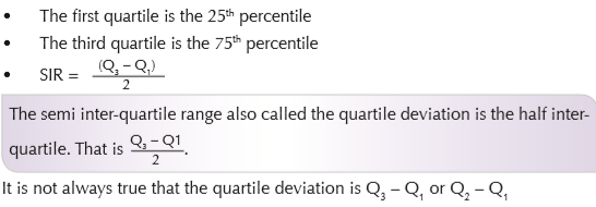

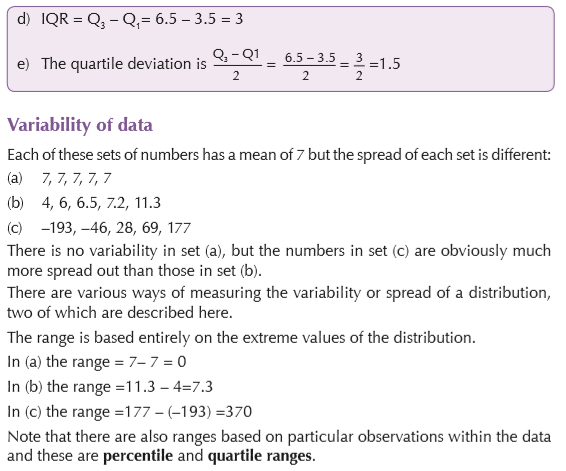
The standard deviation and the variance
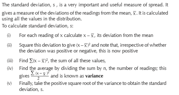
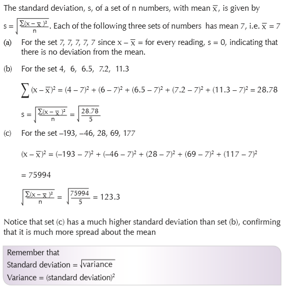
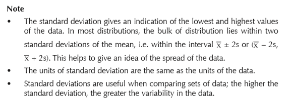
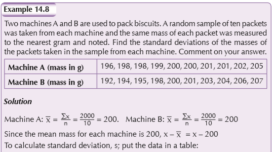
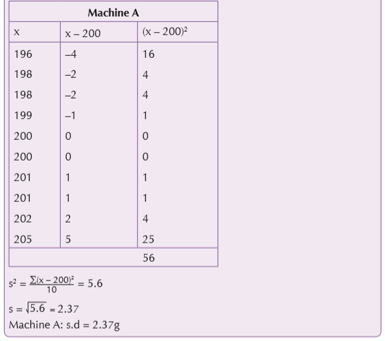
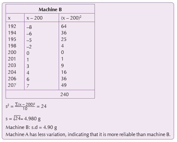
Alternative form of the formula for standard deviation
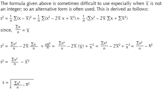
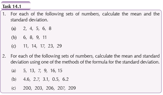
14.3 Coefficient of variation
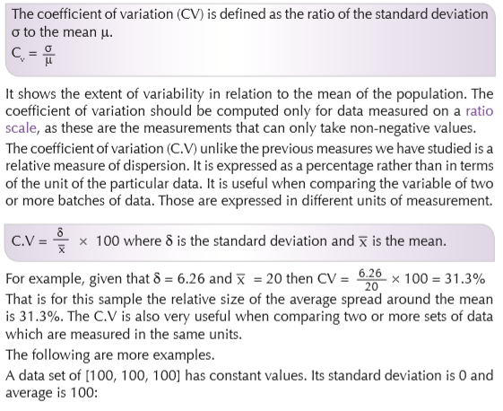
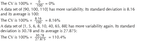
14.4 Application
Activity 14.3
Carry out research to find out real life applications on measures of dispersion. Discuss your findings with the rest of the class.
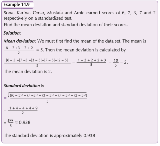
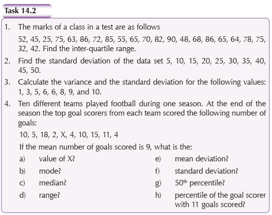

UNIT 15 : Combinatorics
Key unit competence
Use combinations and permutations to determine the number of ways a random experiment occurs.
Learning objectives
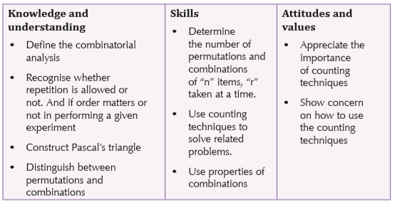
15.1 Counting techniques
Combinatorics , also known as combinatorial analysis, is the area of mathematics concerned with counting strategies to calculate the ways in which objects can be arranged to satisfy given conditions.
Venn diagrams
This is a way of representing sets in a closed curve. They are usually circular or oval shaped. The universal set, written U or , is represented by a rectangle and is a set containing all the sub-sets considered in the problem. In the probability
theory, the universal set is called the sample space and its subsets are called the events.
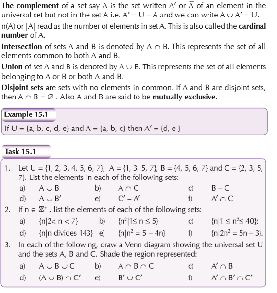
Tree diagrams
A tree diagram is a diagram with a structure of branching connecting lines representing a relationship. It can be used to find the number of possible outcomes of experiments where each experiment occurs in a finite number of ways. For example, when you toss a coin, the outcome is either head or tail. A second toss would also give head or tail. We represent this as:
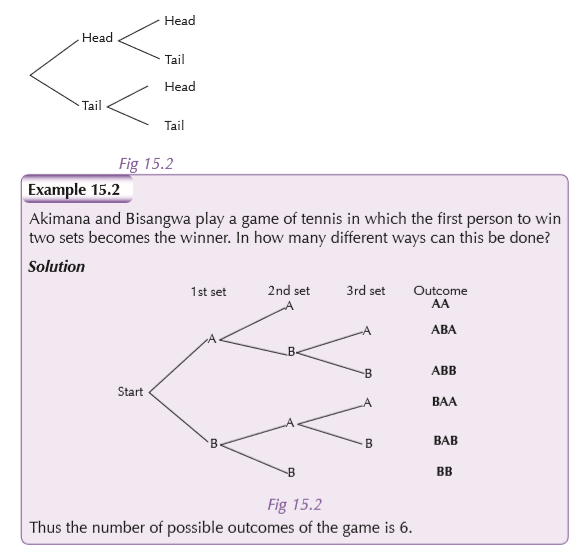
Contingency table
This is a method of presenting the frequencies of the outcomes from an experiment in which the observations in the sample are categorised according to two criteria. Each cell of the table gives the number of occurrences for a particular combination of categories. An example of contingency table in which individuals are categorised by gender and performance is shown below.
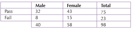
A final column giving the row sums and a final row giving the column sums may be added. Then the sum of the final column and the sum of the final row both equal the number in the sample.
If the sample is categorized according to three or more criteria, the information can be presented similarly in a number of such tables.
Multiplication rule
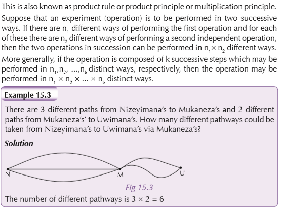
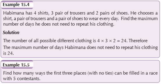
15.2 Arrangements and permutations
Mental task
Imagine that you are a photographer. You want to take a photograph of a group of say 7 people. In how many different ways can they be arranged in a single row?
Factorial notation
Permutations
Activity 15.1
Discuss in groups of 5: in how many different ways can a group of 3 students be arranged to sit in a row?
Share your findings with the rest of the class.
Arrangements without repetition
Suppose that two of the three different pictures, A, B and C are to be hung, in line, on a wall of three places. The pictures can be hung in different orders:

Each of these orders is a particular arrangement of the pictures and is called a permutation.
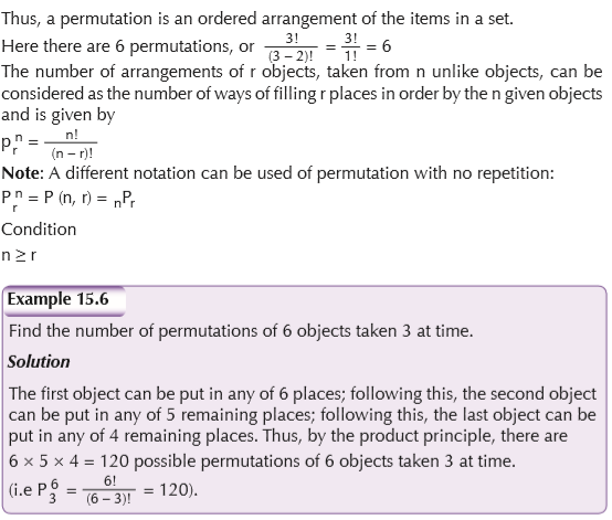
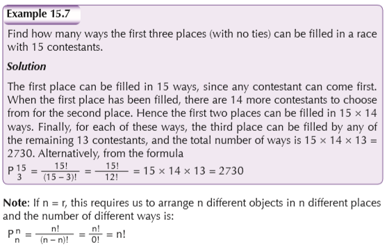
Arrangements with repetition

Arrangement in a circle
Observe the arrangement of four letters A, B, C and D on a circle as shown below

Conditional arrangements
Sometimes arrangements may have certain restrictions which should be dealt with first.
Arrangement with indistinguishable elements
In arranging objects, some sets may contain certain elements that are indistinguishable from each other. Below is how we find the number of arrangements.
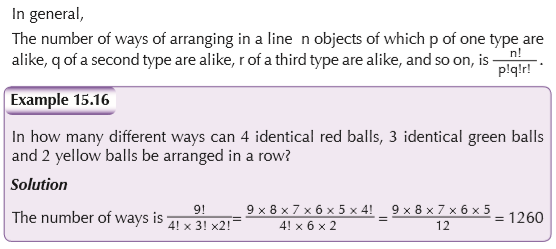
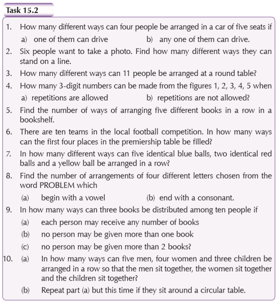
15.3 Combinations
Activity 15.2
Discuss in groups of 5: in how many ways can a committee of 5 students be chosen from a class of 30 students?
Share your findings with the rest of the class.
Definitions and properties


Conditional combination
Sometimes we are given a condition that must be taken into account in a combination.
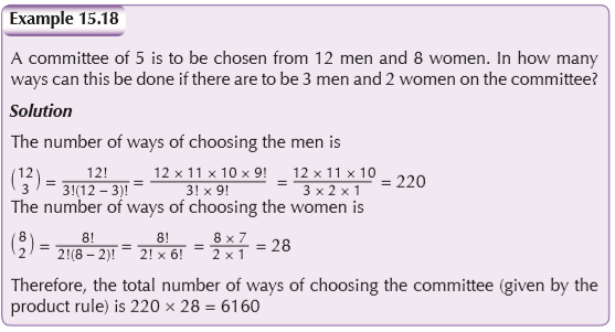
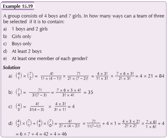
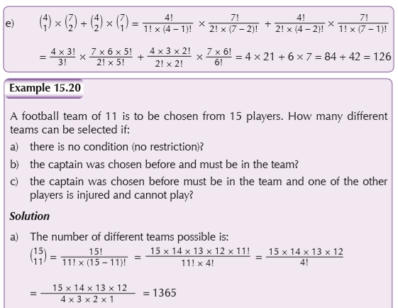
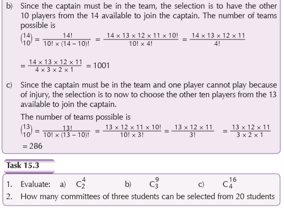
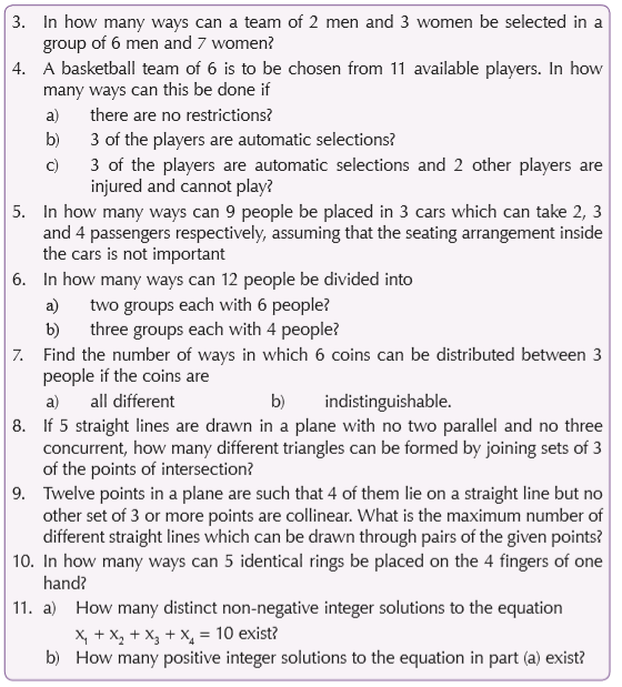
Pascal’s triangles

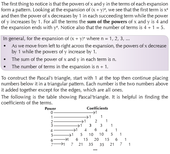
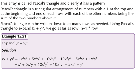
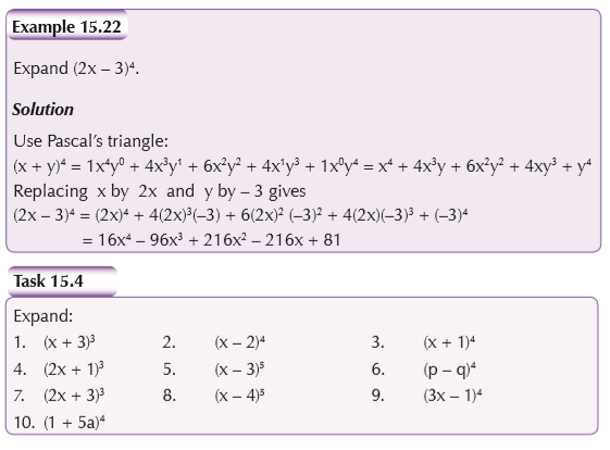
Binomial expansion
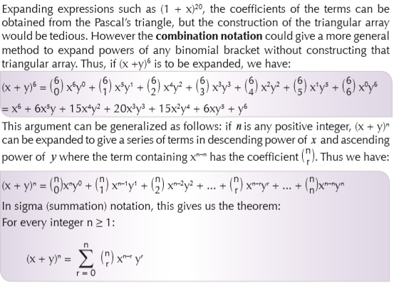
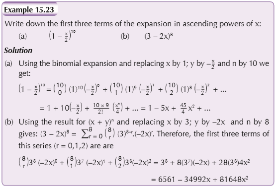

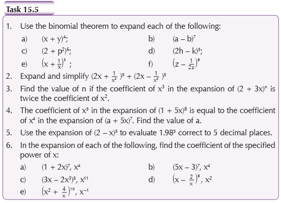
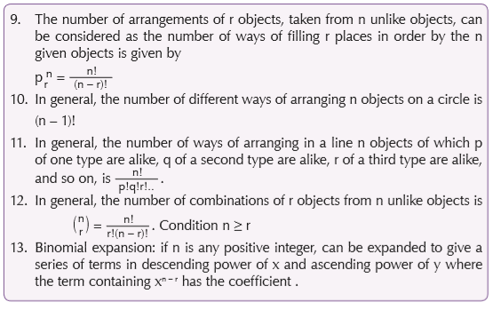
UNIT 16 : Elementary probability
Key unit competence
Use counting techniques and concepts of probability to determine the probability of possible outcomes of events occurring under equally likely assumptions.
Learning objectives
16.1 Concepts of probability
Activity 16.1
In groups, discuss the following.
Have you ever watched people gambling?
What do they rely on to win? What are the problems associated with gambling? Present your findings to the rest of the class.
Many events cannot be predicted with total certainty. The best we can say is how likely they are to happen, using the idea of probability.
Probability
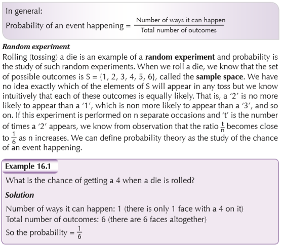
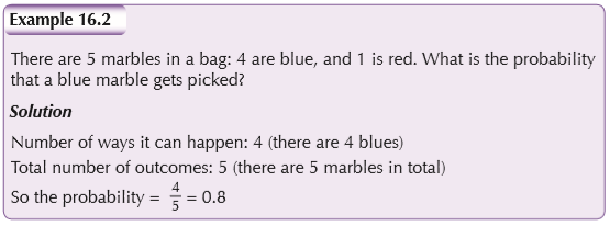
Sample space and events
The set S of all possible outcomes of a given experiment is called the sample space. A particular outcome, i.e., an element of S, is called a sample point. Any subset of the sample space is called an event. The event {a} consisting of a single element of S is called a simple event.
Experiment or trial: an action where the result is uncertain.
Tossing a coin, throwing dice, seeing what fruits people prefer are all examples of experiments.
Sample space: all the possible outcomes of an experiment
Choosing a card from a deck
There are 52 cards in a deck (not including Jokers) So the sample space is all 52 possible cards: {Ace of Hearts, 2 of Hearts, and so on... }
Event: a single result of an experiment
• Getting a Tail when tossing a coin is an event
• Rolling a “5” is an event. An event can include one or more possible outcomes:
• Choosing a “King” from a deck of cards (any of the 4 Kings) is an event • Rolling an “even number” (2, 4 or 6) is also an event
Anne wants to see how many times a “double” comes up when throwing 2 dice. Each time Anne throws the 2 dice is an experiment. It is an experiment because the result is uncertain.
The event Anne is looking for is a “double”, where both dice have the same number. It is made up of these 6 sample points:
(1,1), (2,2), (3,3), (4,4), (5,5) and (6,6) or S ={(1,1), (2,2), ... .}
The sample space is all possible outcomes (36 sample points):
(1,1), (1,2), (1,3), (1,4) ... (6,3), (6,4), (6,5), (6,6)
Probability of an event under equal assumptions
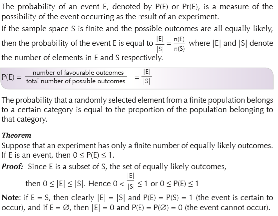
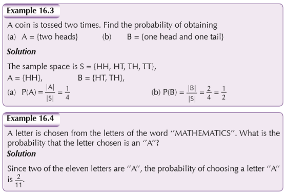
Complementary event
If E is an event, then E’ is the event which occurs when E does not occur. Event E and E’ are said to be complementary events.
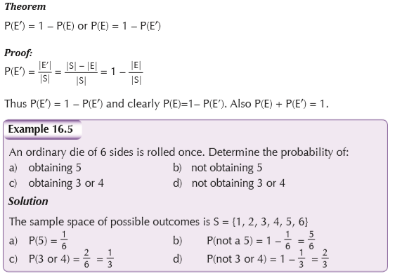
Consider two different events, A and B. which may occur when an experiment is performed. The event A ∪ B is the event which occurs if A or B or both A and B occurs, i.e.. at least one of A or B occurs.
The event A ∩ B is the event which occurs when both A and B occurs.
The event A – B is the event which occurs when A occurs and B does not occur.
The event A′ is the event which occurs when A does not occur.
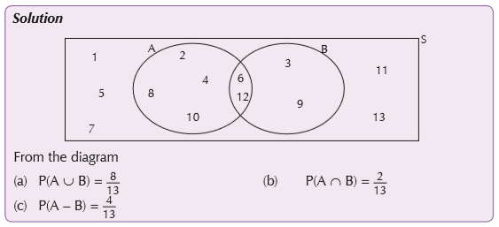
Permutations and combinations in probability theory
Activity 16.2
Discuss the following scenario in groups and present your findings to the rest of the class.
If there are 4 women and 3 men and you wanted them seated in a row, what is the probability that the men will be seated together?
Permutations and combinations can be used to find probabilities of various events particularly when large sample sizes occur. In everything we do, we have to use the formula
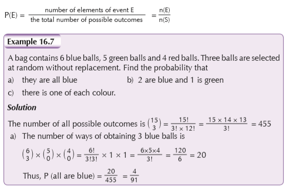
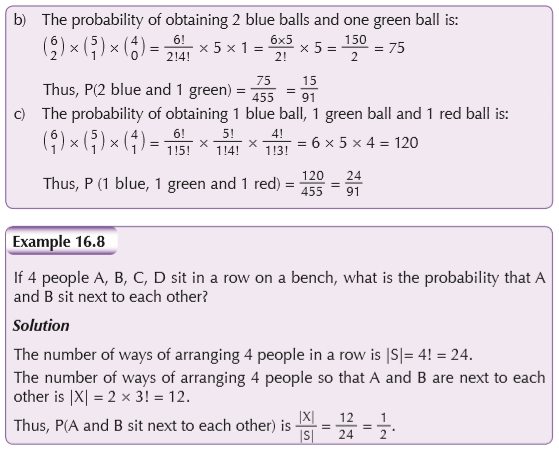

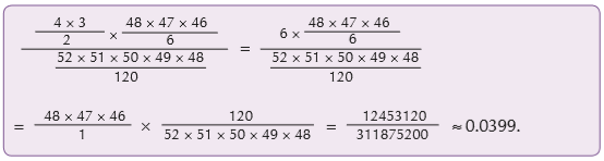
16.2 Finite probability spaces
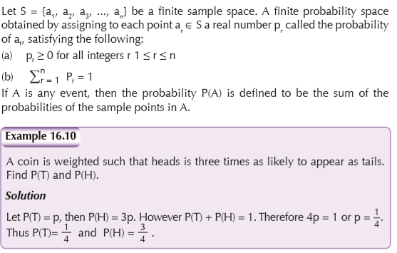
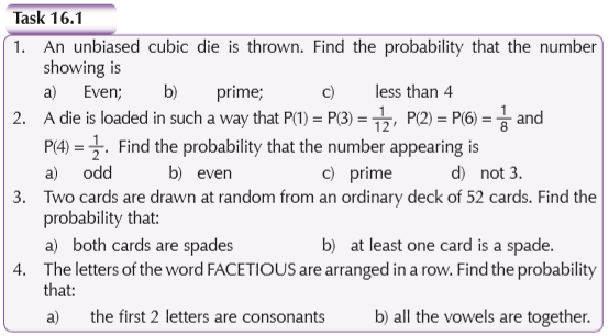
16.3 Sum and product laws
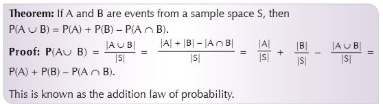
Mutually exclusive events
Events A and B are said to be mutually exclusive if the events A and B are disjoint i.e. A and B cannot occur at the same time.
For mutually exclusive events, A ∩ B = ∅. P(A ∩ B) = P(∅) = 0; and so the addition law reduces to P(A ∪ B) = P(A) + P(B).
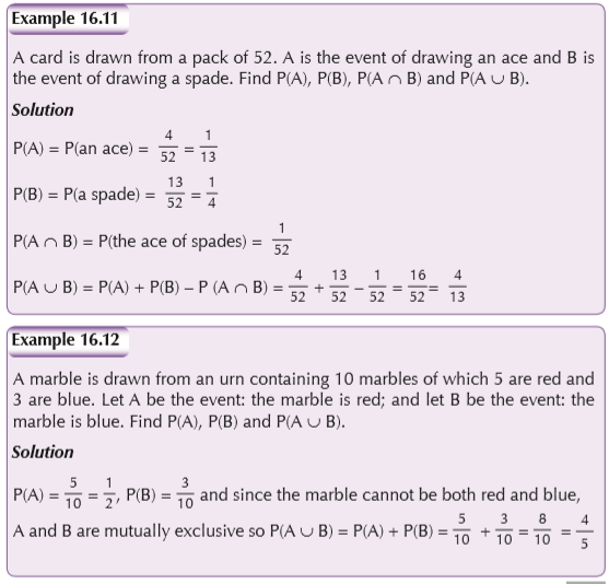
Independent events
Two events are independent if the occurrence or non occurrence of one of them does not affect the occurrence of the other. Otherwise, A and B are dependent. For independent events, the probability that they both occur is given by the Following product law:
P(A ∩ B) = P(A) × P(B)

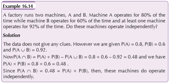
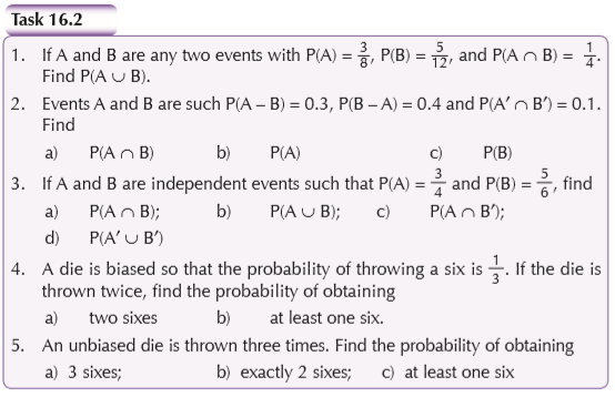
16.4 Conditional probability
The probability of an event B occuring given that A has occurred is called the conditional probability of B given A and is written P(B|A).
Here P(B|A) is the probability that B occurs considering A as the sample space, and since the subset of A in which B occurs is A ∩ B, then

The general statement of the multiplication law is obtained by rearranging this result:
P(A ∩ B) = P(A) × P(B|A)
Thus the probability that the two events will both occur is the product of the probability that one will occur and the conditional probability that the other will occur given that the first has occurred. As A and B are interchangeable, we can also write P(A ∩ B) = P(B) × P(A|B)
If A and B are independent, then the probability of B is not affected by the occurrence of A and so P(B|A)=P(B) giving P(A ∩ B) = P(A) × P(B) which is our definition of independence.
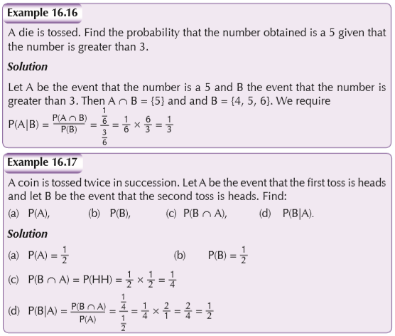
A tree diagram can be quite useful in the calculation of certain probabilities. The following example illustrates the method.