UNIT 8 : Limits of polynomial, rational and irrational functions
Key unit competence
Evaluate correctly limits of functions and apply them to solve related problems.
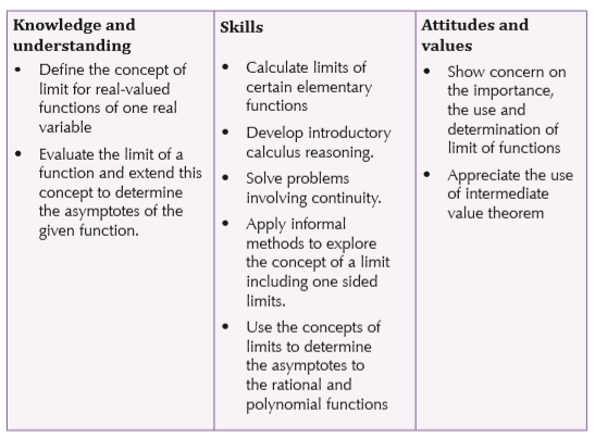
Learning objectives
8.1 Concept of limits
Neighbourhood of a real number
Activity 8.1
You have heard about the term ‘neighbourhood’ in everyday life. What does it mean?
Carry out research to find the meaning of the term in mathematics. Discuss your findings in class. Use diagrams in your explanations.
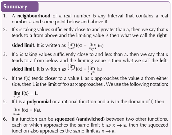
By a neighbourhood of a real number c we mean an interval which contains c as an interior point.
On the real line, a neighborhood of a real number is an open interval (a – δ, a + δ) where δ > 0, with its centre at a. Therefore, we can say that a neighborhood of the real number is any interval that contains a real number a and some point below and above it.
We can add:
Let x be a real number. A neighbourhood of x is a set N such that for some ε > 0 and for all y, if |x − y| < ε then y ∈ N.
Limit of a variable
Activity 8.2
In groups of five, work out the following:
Let f(x) = 2 x + 2 and compute f(x) as x takes values closer to 1. First consider values of x approaching 1 from the left (x < 1) then consider x approaching 1 from the right (x > 1).
In Activity 8.2, x approaching 1 from the left (x < 1) gives us:

and x approaching 1 from the right (x > 1) gives us:
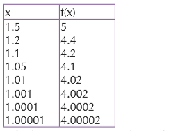
In both cases as x approaches 1, f(x) approaches 4. Intuitively, we say that

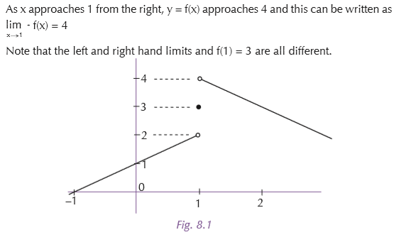
Note: We are talking about the values that f(x) takes when x gets closer to 1 and not f(1). In fact we may talk about the limit of f(x) as x approaches a even when f(a) is undefined.
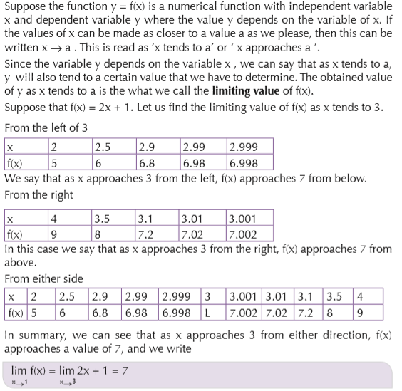
If f(x) can be made as close as we like to some number a by making x sufficiently close to (but not equal to) a, then we say that f(x) has a limit of L as x approaches a, and we write

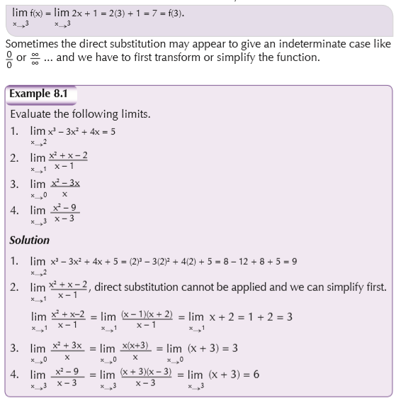
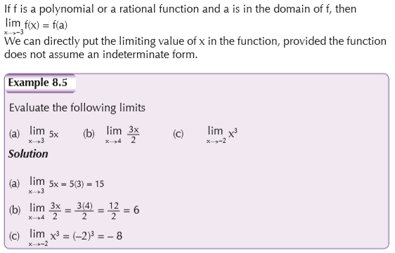
Note that in the above case the limit is found by the direct substitution i.e.
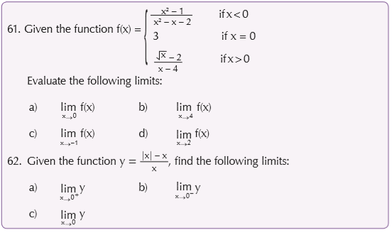
One-sided limits
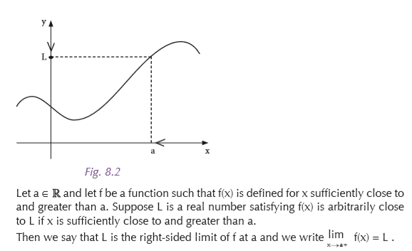
Right-sided limits
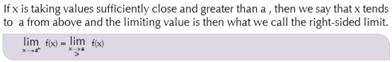
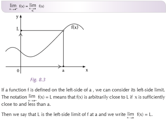
Left-sided limits
If x is taking values sufficiently close to and less than a, then we say that x tends to a from below and the limiting value is then what we call the left-sided limit. It is written as:
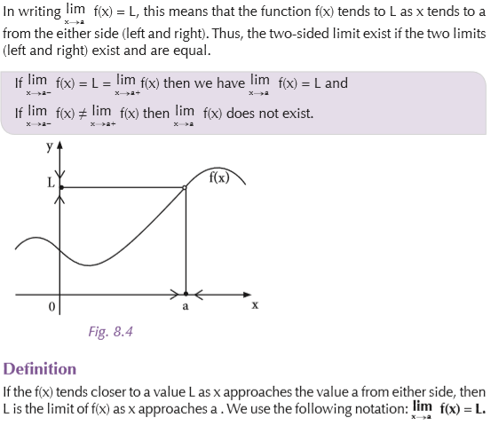
Two-sided limits
Evaluation of algebraic limits by direct substitution
Infinity limits
Let f be a function defined on both sides of a, except possibly at a itself. Then

means that the values of f(x) can be made arbitrarily large (as large as we please) by taking x
sufficiently close to a, but not equal to a.
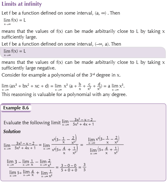
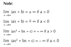
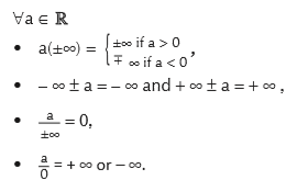
Note: To compute the limit of a function as x → ±∞, we use the following principles
8.2 Theorems on limits
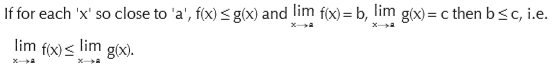
Compatibility with order
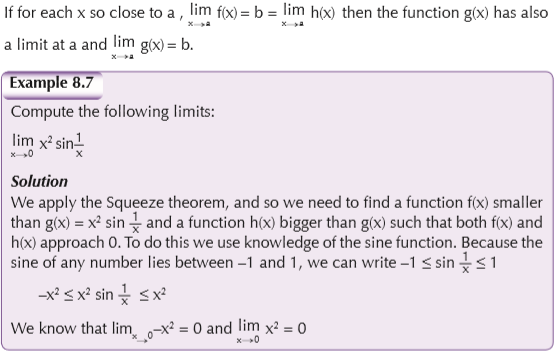
Squeeze theorem
This is also known as the sandwich theorem, comparison theorem or vice theorem. If a function can be squeezed (sandwiched) between two other functions, each of which approaches the same limit b as x → a , then the squeezed function also approaches the same limit as x → a.
Let f(x), g(x) and h(x) be three functions such that f(x) ≤ g(x) ≤h(x).
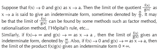
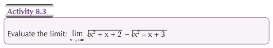
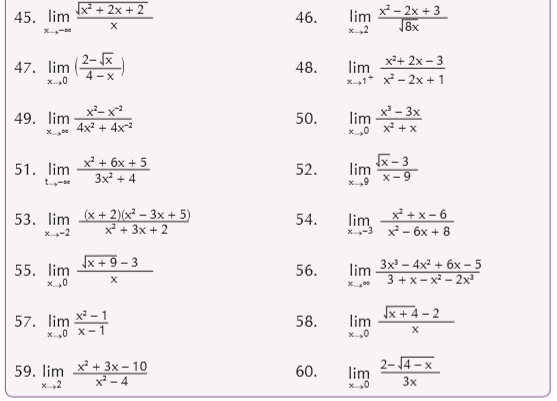
8.3 Indeterminate forms
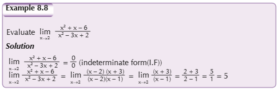
Method of factors

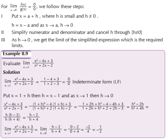
Method of substitution
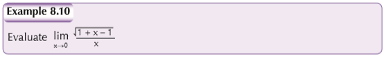
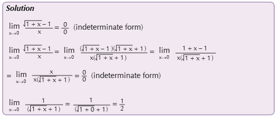
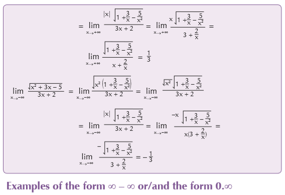
Method of rationalisation
In functions which involve square roots, rationalisation of either numerator or denominator and simplifications will facilitate the work.
True value of limits
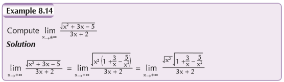
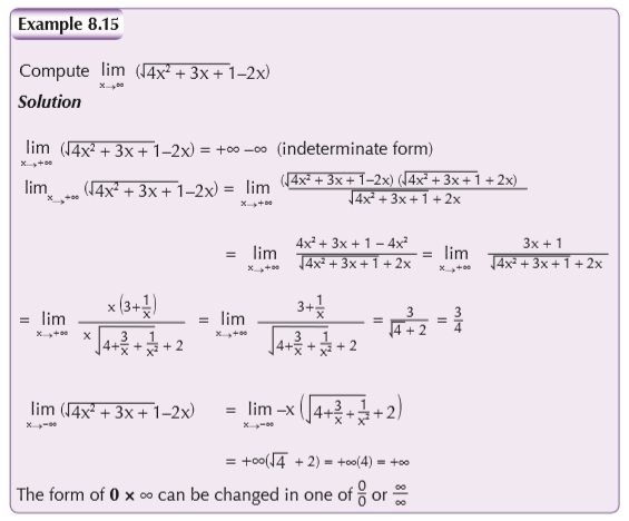
Computation of limits may results in indeterminate form (I.F) such as

Thus, we we can say that:
• If the degree of the numerator is smaller than the one of the denominator, the limit of the fraction as x → ∞ is zero;
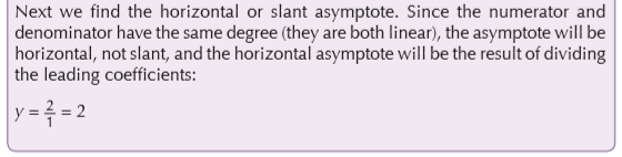
• If the degree of the numerator is equal to the one of the denominator, the limit of the fraction as x → ∞ is equal to the quotient of the coefficient of the terms with the highest power;
• If the degree of the numerator is greater than the one of the denominator, the limit of the fraction as x → ∞ gives infinite (the sign of infinite depends on the highest power and its coefficient).
8.4 Application of limits
Activity 8.4
In groups, carry out research to find out the applications of limits. Discuss your findings with the rest of the class.
Continuity of a function at a point or interval
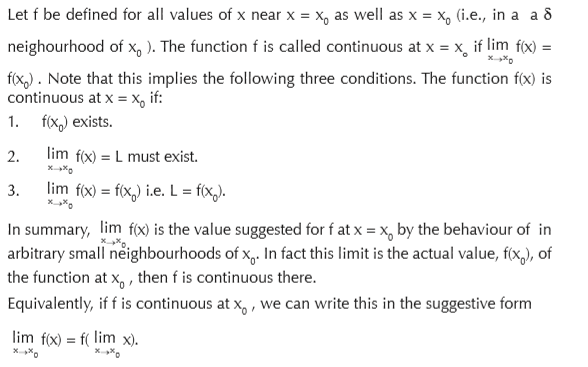
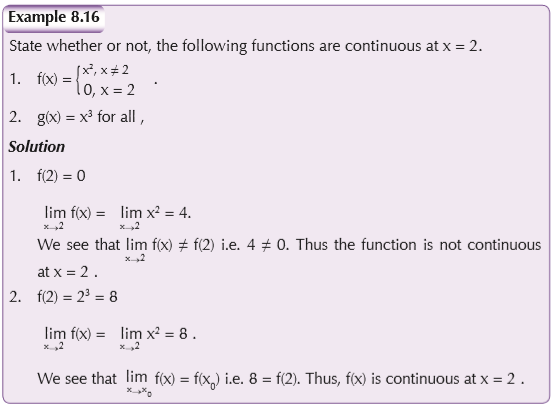
Points where f fails to be continuous are called discontinuities of f and f is said to be discontinuous at these points.
Continuity over an interval
The function is said to be continuous over interval ]a, b[ if and only if f(x) is continuous at any point of the interval ]a, b[. i.e.
f is continuous for all x0 ∈]a, b[. f is continuous at the right side of a. f is continuous at the left side of b .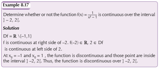
Properties1. The sum of two continuous functions is a continuous function.
2. The quotient of two continuous functions is a continuous function where the denominator is not zero.Asymptotes
Activity 8.5
What is an asymptote? Carry out research and find out the meaning. Also, find out the types of asymptotes.
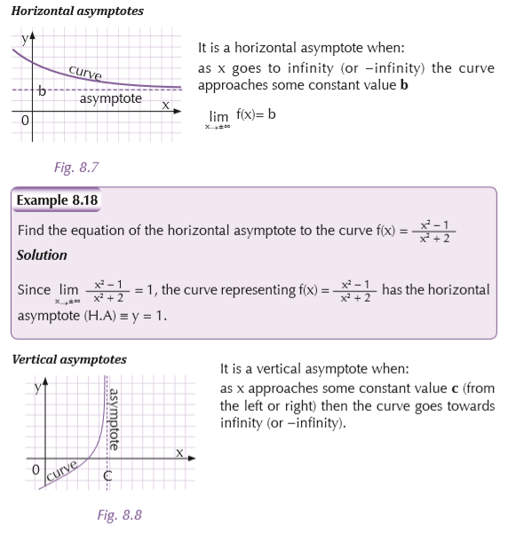
An asymptote is a line that a curve approaches, as it heads towards infinity:
Types
There are three types of asymptotes: horizontal, vertical and oblique:

An asymptote can be in a negative direction, the curve can approach from any side (such as from above or below for a horizontal asymptote), or may actually cross over (possibly many times), and even move away and back again.
The important point is that: The distance between the curve and the asymptote tends to zero as they head to infinity (or−infinity)
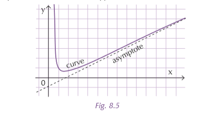
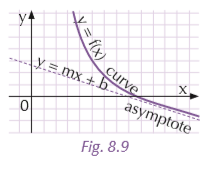
Oblique asymptotes
It is an oblique asymptote when: as x goes to infinity (or −infinity) then the curve goes towards a line y = mx + b
(note: m is not zero as that is a horizontal asymptote).
The characteristics of the three kinds of asymptotes: vertical asymptote, horizontal asymptote and oblique asymptote are:
Note: For the rational functions;
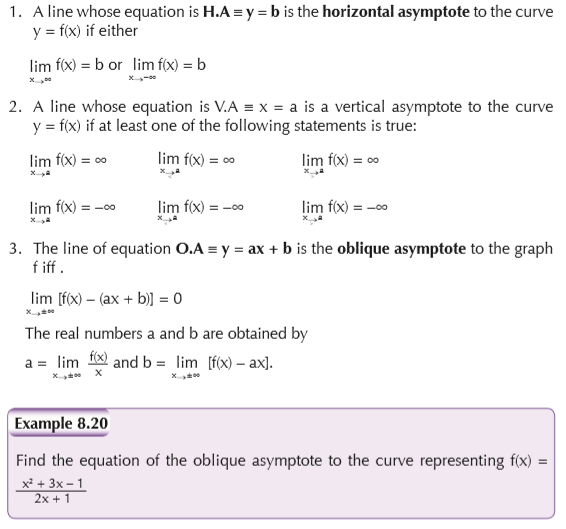
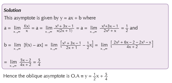
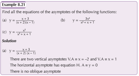
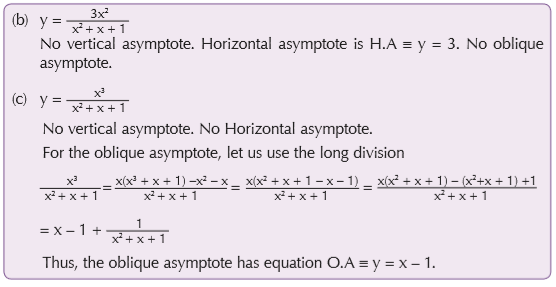
- There is the oblique asymptote if the degree of the numerator is one greater than the degree of the denominator. An alternative way to find the equation of the oblique asymptote is to use a long division. There the equation is simply the quotient.
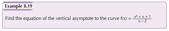
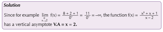
- The vertical asymptote, are found to be the values that make the denominator zero
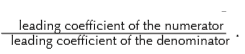
- For the horizontal asymptote, if the degree of the numerator is less than the degree of the denominator, then H.A ≡ y = 0. If the degree of the numerator is or equal to the degree of the denominator, then H.A ≡ y =
- The horizontal asymptote is the special case of the oblique asymptote.
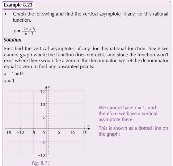
Graphing asymptotes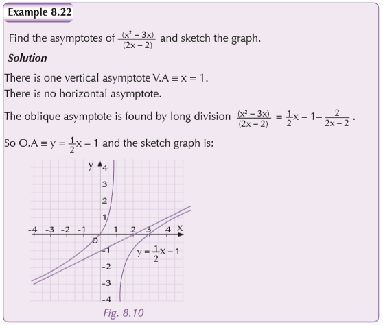
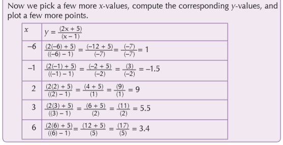
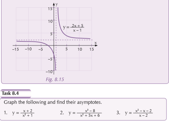
To graph a rational function, you find the asymptotes and the intercepts, plot a few points, and then sketch in the graph.