UNIT 3:ADVANCED SPREADSHEET I
Introductory activity 3
At the end of the year Teacher Peace was overloaded with work as she was
required to prepare the end of the year report for pupils. The marks given to her
are word softcopies for which total are manually. She has the task to write the
marks in the word sheets, calculate the totals for the whole year, the average per
subject for the whole year and the overall average for the whole year for each
pupil. For this reason she is planning to buy a calculator and is considering hiring
someone to help her which is against the ethics.
a. Advise Teacher Peace on how to handle this situation using
the word files she has
b. Advise this same teacher on how excel program can helpher
c. Comp are the easiness of the task when Teacher Peace
adopts the advice in a) and when she chooses the optionpresented in b
3.1. Conditional formatting
Activity 3.1
Open Spreadsheet program and enter data in the table below. Save thefile as “Burera Ltd Sales data”
Do the followings: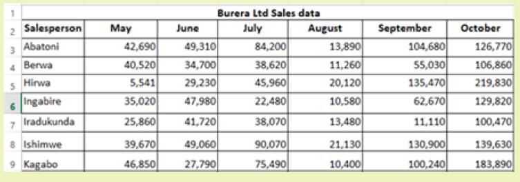
1. Using Burera Ltd Sales data, show salespersons who are meeting
their monthly sales goals. The sales goal is 50,000 items per month
2. Highlight all salesperson whose sales are below the average
3. Highlight with blue color ,all salesperson whose sales are above80,000
Conditional formatting is a spreadsheet functionality which allows Excel(spreadsheet)
users to specify conditions allowing to get specific answers on data in the worksheet
that was otherwise not easy to analyze.
It can be applied to a range of cells or an entire worksheet and makes cells meeting
specified criteria have relative formatting (font). If the formatting condition is true,
the range of cells is formatted according to the preset criteria, else that range is not
formatted.
Conditional formatting is a feature in many spreadsheet applications that allows
users to apply specific formatting to cells that meet certain criteria. It is most often
used as color-based formatting to highlight, emphasize or differentiate among data
and information stored in a spreadsheet.
Conditional formatting enables spreadsheet users to do a number of things. It calls
attention to important data points such as deadlines and at-risk tasks. It can also
make large data sets more digestible by breaking up the wall of numbers with
a visual organizational component. Among the options provided by conditional
formatting are: highlight cell rules, top bottom rules, customized rules, etc
3.1.1. Highlight cell rule
Conditional formatting can be used to enhance the reports and dashboards
in Excel. The conditional formatting statement under the Highlight Cells Rules
category allow to highlight the cells whose values meet a specific condition.
The benefit of a conditional formatting rule is that Excel automatically reevaluates
the rule each time a cell is changed provided that cell has a conditional formatting
rule applied to it. Those rules include: greater than, less than, equal to, between,
text that contain, A Date occurring, duplicate values, …Here are the steps to apply the highlight cell rule:
Step 1: Select the desired cells on which to apply the conditional formatting rule
Step 2: From the Home tab, click the Conditional Formatting command. A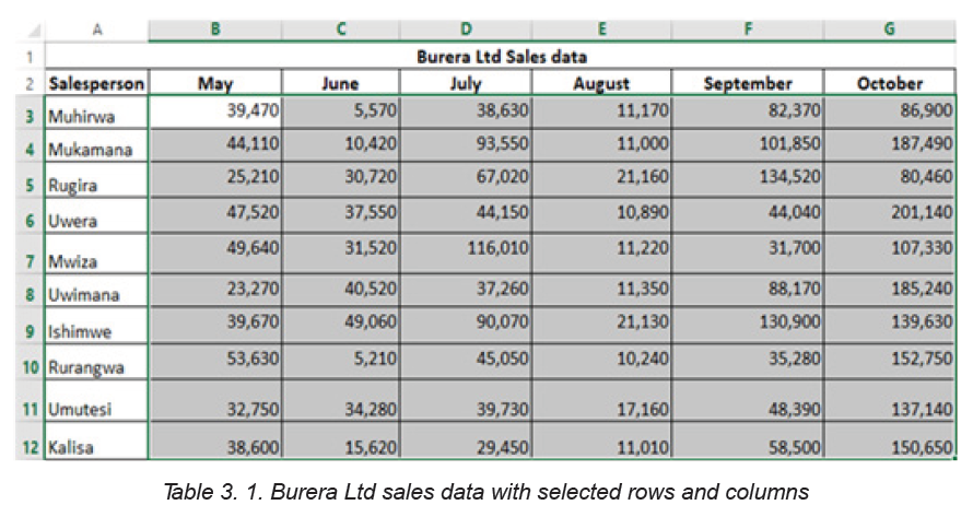
drop-down menu will appear.
Step 3: Hover the mouse over the desired conditional formatting type, and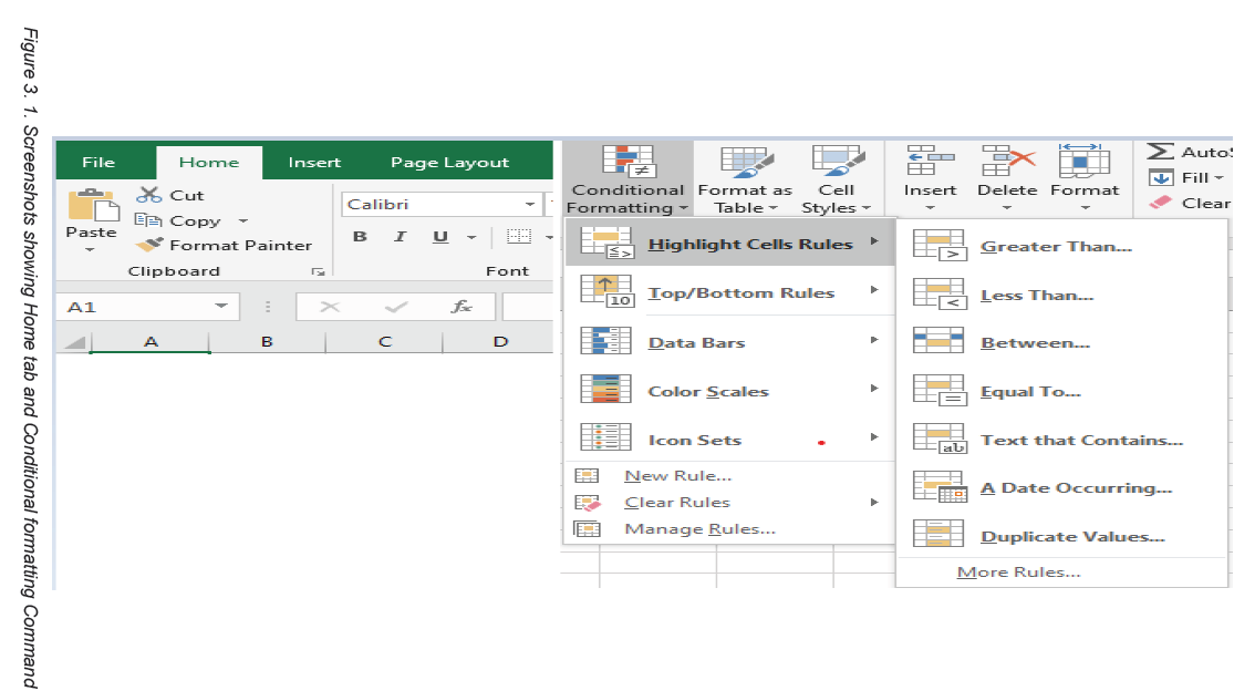
then select the desired rule from the menu that appears. In the Activity 4.1, cells
that are greater than 50, 000 are to be highlighted.
Step 4: A dialog box will appear. Enter the desired value(s)into the blank field.
In the case of the activity 4.1.the taken value is 50, 000.
Step 5: Select a formatting style from the drop-down menu. In the Activity3.1, the color to choose is Green Fill with Dark Green Text, then click OK.
Step 6: The conditional formatting will be applied to the selected cells. In this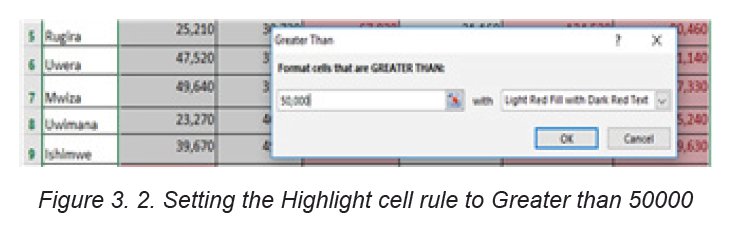
case, it’s easy to see which salesperson reached the 50, 000 sales goalsfor each month.
Note: It is possible to apply multiple conditional formatting rules to a cell range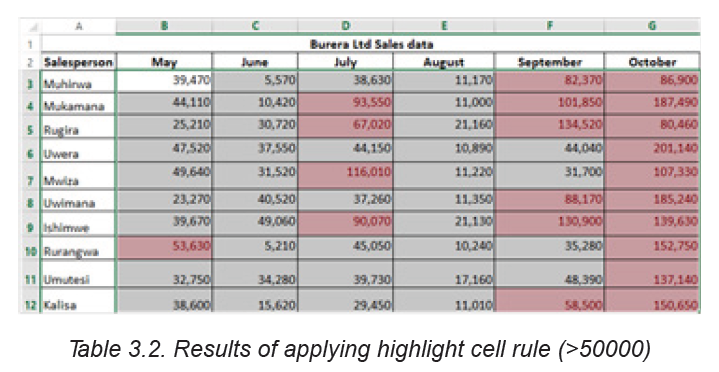
or worksheet. This allows to visualize different trends and patterns in data.
3.1.2. Clear rule
Rules that have been used to highlight cells that meet certain conditions can be
removed and have text with no highlight when the rules are no longer needed
or when there is a need to set new rules.
To clear rules, do the following:
Step 1: Select the desired cells for clearing the conditional formatting rule Step 2:
On the Home tab, in the Styles group, click Conditional Formatting Step 3: ClickClear Rules then click Clear Rules from Selected Cells
After clearing rules for selected cells, cells are no longer colored, there is no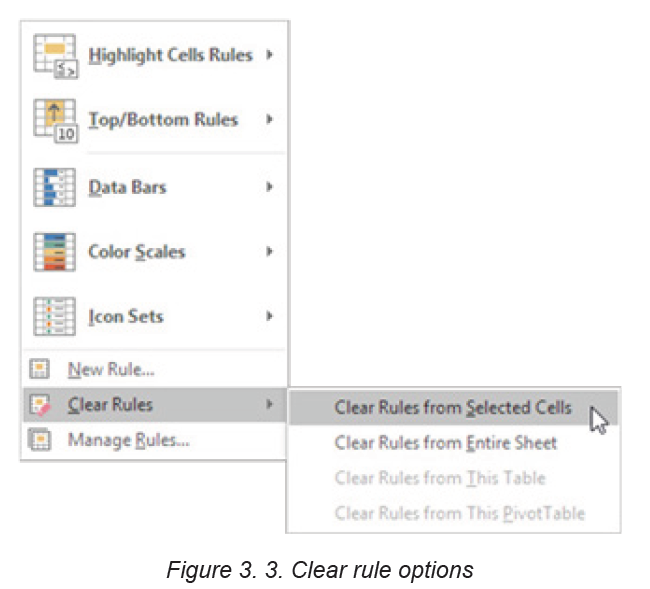
more formatting in cells.
3.1.3. Create Top/Bottom Rules
Top/Bottom rules are another useful Conditional Formatting in Excel. These rules
allow users to call attention to the top or bottom range of cells, which can be specified
by number, percentage, or average. The steps to create Top/Bottom rules are:
Step 1: Select the desired cells for the conditional formatting rule
Step 2: From the Home tab, Select Conditional Formatting then Top/BottomRules then click Above Average
Step 3: A dialog box will appear. Choose color format to use like “Light Red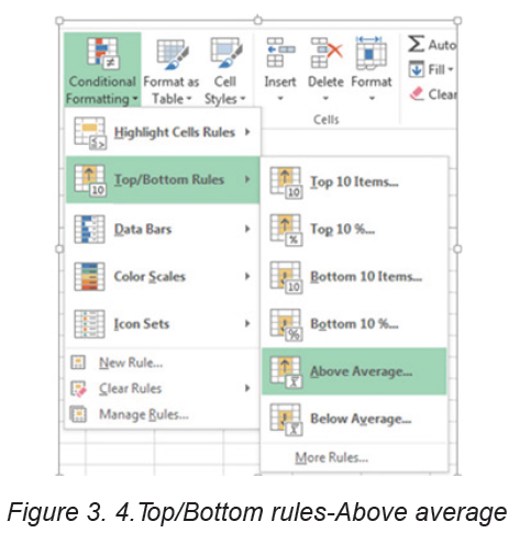
Fill with Dark Red text”.After choosing cells format, Press “OK”
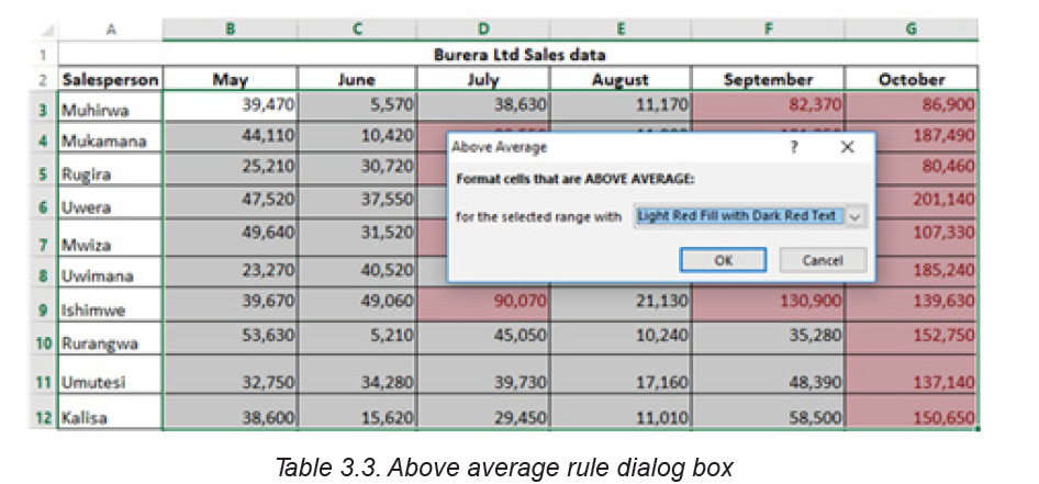
Step 4: The sheet will now highlight the values above the average
3.1.4. Create new rule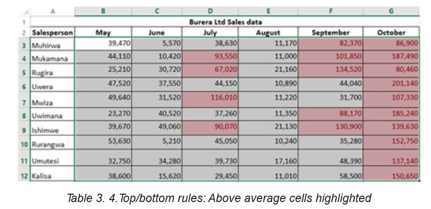
Excel allows to create a formula-based conditional formatting rule. The available
options are:
• Formatting cells based on their values,
• Formatting cells that contain certain values,
• Formatting only top or bottom ranked values,
• Formatting only values that are below or above average,
• Formatting only unique or duplicate values and using a formula to determinewhich values to format.
All those options are presented in the window below:
Step 1: Select the cells to be formatted. In the Home tab click on Conditional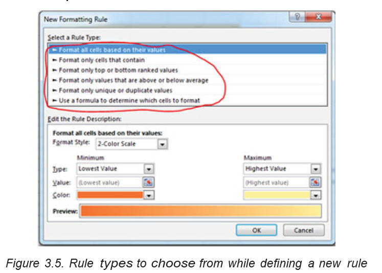
Formatting command and click New rule.
Step 2: Create a conditional formatting rule, and select the Formula option then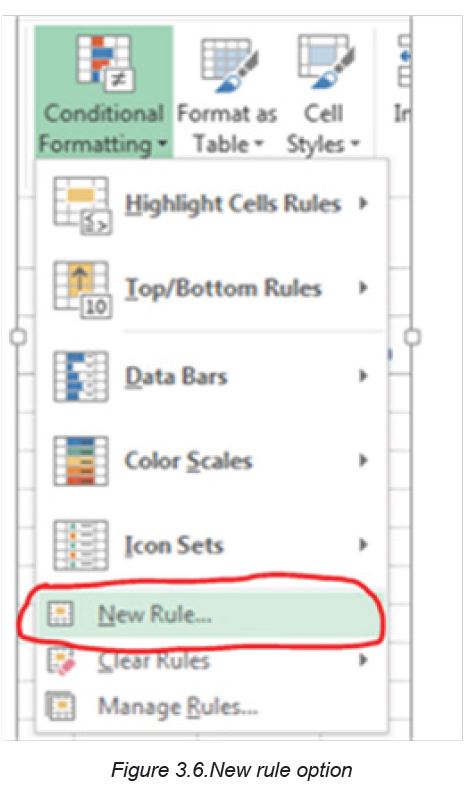
click OK. In the window below the option “Use a formula to determine which
cells to format” has been chosen
1. Format all cells based on their values
Step 1: New formatting rule window will be opened.
Step 2: Select Format all cells based on their values option, however this isby default selected.
There are at least four format styles that can be applied while applying conditional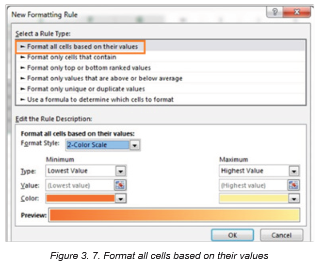
formatting on Excel data. Those formats are: Data Bar, Icon Set,
2-Color Scale and 3-Color Scale
a. 2-color scale
Step 1: Choose minimum and maximum valuesStep 2: Click Ok button to apply this conditional formatting
Step 3: Data set with this condition formatting will look like below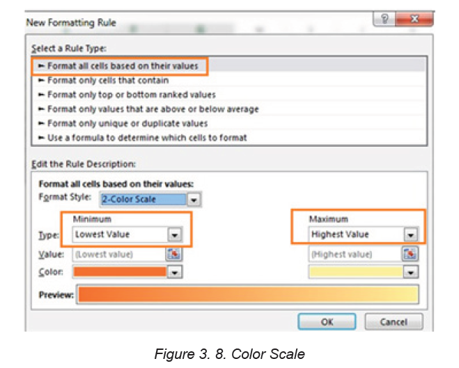
Note: we have chosen minimum number to 50,000 and the maximum to80,000, then selected a colors to separate both values.
b. 3-color scale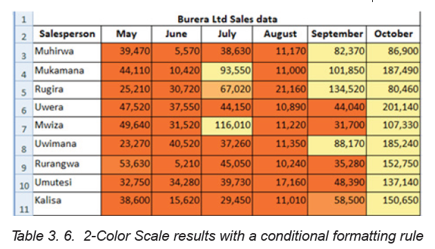
Step 1: New formatting rule window will be opened.
Step 2: Select Format all cells based on their values option, however this isby default selected.
Below are steps to apply 3 -color formatting style: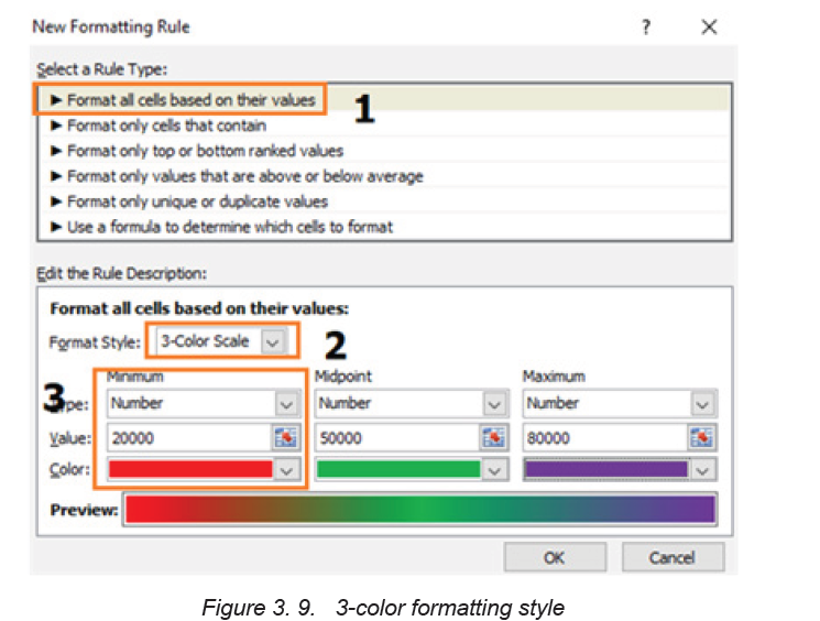
Step 3: Select 3 color scale option in format style
Step 4: Choose the type; here we are taking as Minimum, Midpoint and
Maximum
Step 5: Put values for number for Minimum, Midpoint and Maximum then,results are displayed as follows:
2. Use a formula to determine which cells to format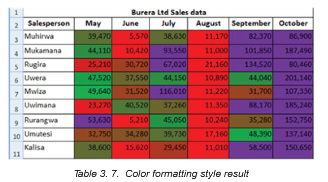
New rules can be created by customizing own formulas. By using custom
made formula, a custom condition that triggers a rule is created and can be
applied as the user needs it to be applied. In the data that is going to be used
the formula = B3>80000 has been applied for formatting.
To specify the formatting formula click on Conditional Formatting tab then New
Rule and choose Use Formula to determine which cells to format as in thewindow below:
Step 3: In the window that will appear, enter a formula that returns TRUE or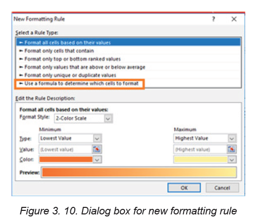
FALSE then set formatting options, save the rule and press OK
After clicking OK cells that meet the formatting rule are highlighted as specified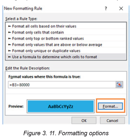
in the new rule. In the window below cells meeting the criteria are blue coloredas it has been specified in the preceding window.
Note: Always write the formula for the upper-left cell in the selected range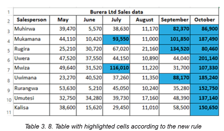
and Excel will automatically copy the formula to the other cells in the selected
range.
Below are some formulas that apply conditional formatting and return TRUE or
FALSE, or numeric equivalents that can be used in setting formatting cell rules
based on formula:
1. =ISODD (A1): This function is used to check if a numeric value is an odd
number. ISODD returns TRUE when a numeric value is odd and FALSE when
a numeric value is even. If value is not numeric, ISODD will return the #VALUE
error.
2. =ISNUMBER (A1): The function is used to check if a value is a number.
ISNUMBER will return TRUE when value is numeric and FALSE when not.
3. AND (A1>100, B1<500): The AND function is used to apply more than
one condition at the same time, up to 255 conditions. Each logical condition
(logical1, logical2, etc.) must return TRUE ExamplesAND (A1>100, B1<500) tests if the value in A1 is greater than100 and B1 less than 500
APPLICATION ACTIVITY 3.1
Open the file “Burera Ltd. Sales Data”
1. Using Burera Ltd Sales data, show salespersons who are not meeting
their monthly sales goals. The sales goal is 50,000 item per month
2. Highlight all salesperson whose sales are above the average
3. Highlight with green color all salesperson whose sales are below
80,000
3.2 Charts
Activity 3.2
1.Open Spreadsheet program, en- ter data in the table below and saveit as “Production”
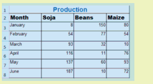
2.Using Production data make the graph below:
3.2.1 Create a Chart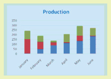
In spreadsheet, a chart is often called a graph. It is a visual representation of data
from a worksheet that can bring more understanding to the data than just looking
at the numbers.
A chart is a powerful tool that allows to visually display data in a variety of
different chart formats such as: Bar, Column, Pie, Line, Area, and many.
In order to create a chart, the following steps are followed:
Step 1: Select the desired cells in the chart creation
1.Open Spreadsheet program, en- ter data in the table below and save it as“Production”
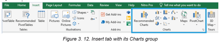
Step 2: On the Insert tab, in the Charts group, choose the type of chart to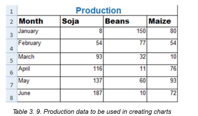
use. In this case the type chosen is the column chart. Click the column chartsymbol
Step 3: Choose the appropriate style. Here a Column Chart has been
chosen. The chart looks like in the image below:
3.2.2. Change Legend Position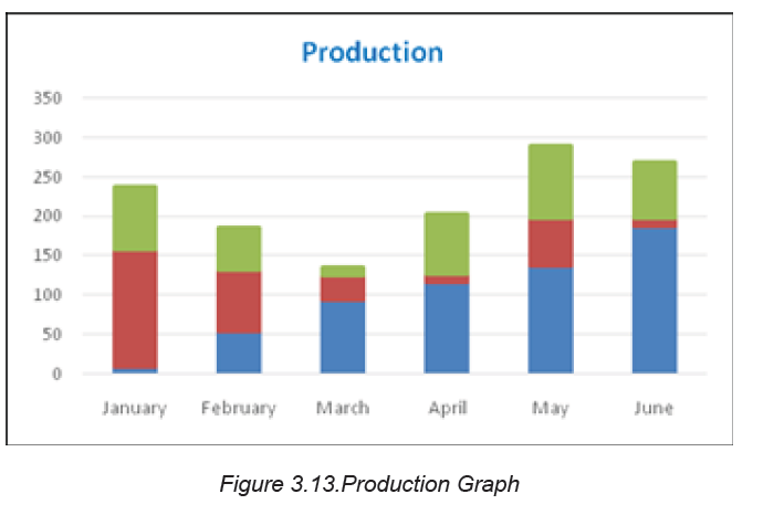
To move the legend to the right side of the chart, go through the following steps.
Step 1: Select the chart.
Step 2: Click the button on the right side of the chart, choose Legend and
click on the arrow next to it. Click on any option to apply in this case Rightwas chosen.
After changing the Legend style, the Legend will be located on the right side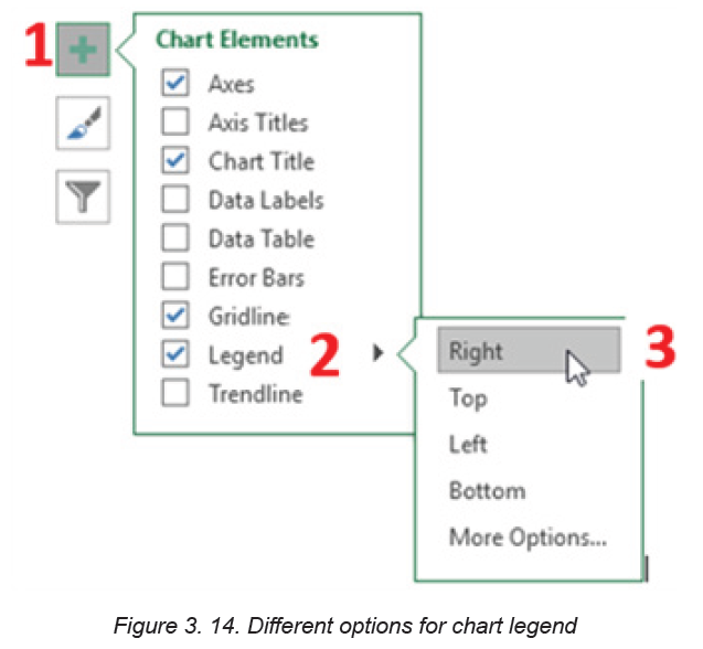
of the chart as it was specified in the steps. The chart looks like in the imagebelow:
3.2.3. Data Labels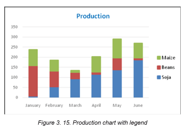
Data labels focus the readers’ attention on a single data series or data point.
These labels can be arranged in the center of the bar, outside end or any
other fashion that the reader wants. Data labels positions are set in this way:
Step 1: After selecting the chart click a green bar to select the Data Labels.
Step 2: Choose the position where data is going to appear, in this caseCenter has been chosen
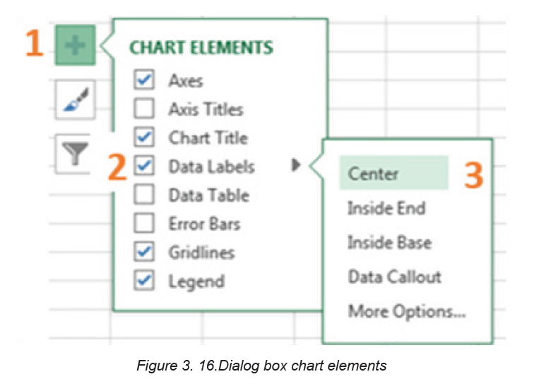
The graph below with data labels in centers is the result:
3.2.4 Change Chart Type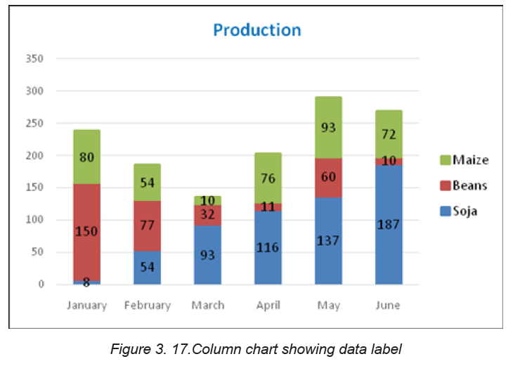
There are different types of chart which can be used depending on the data
to display. Switching from one chart type to another is done in this way:
Step 1: Select the chart for which the type is to be changed
Step 2: Click on the Design tab found under the Chart Tools and in theType group, click Change Chart Type.
Step 3: In the new window that will appear click on either“Recommended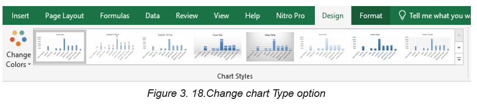
Charts”or “All Charts”. Choosing all charts will display all the charts from
which user can choose. In the image below the line chart was chosen. Selectthe type and click OK
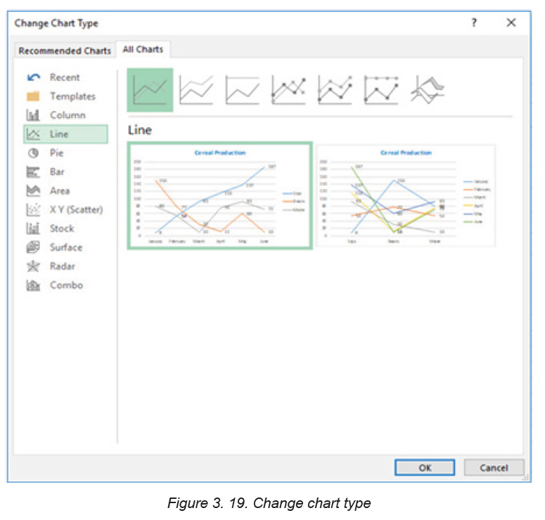
The resulting graph will look like in the image below:
APPLICATION ACTIVITY 3.2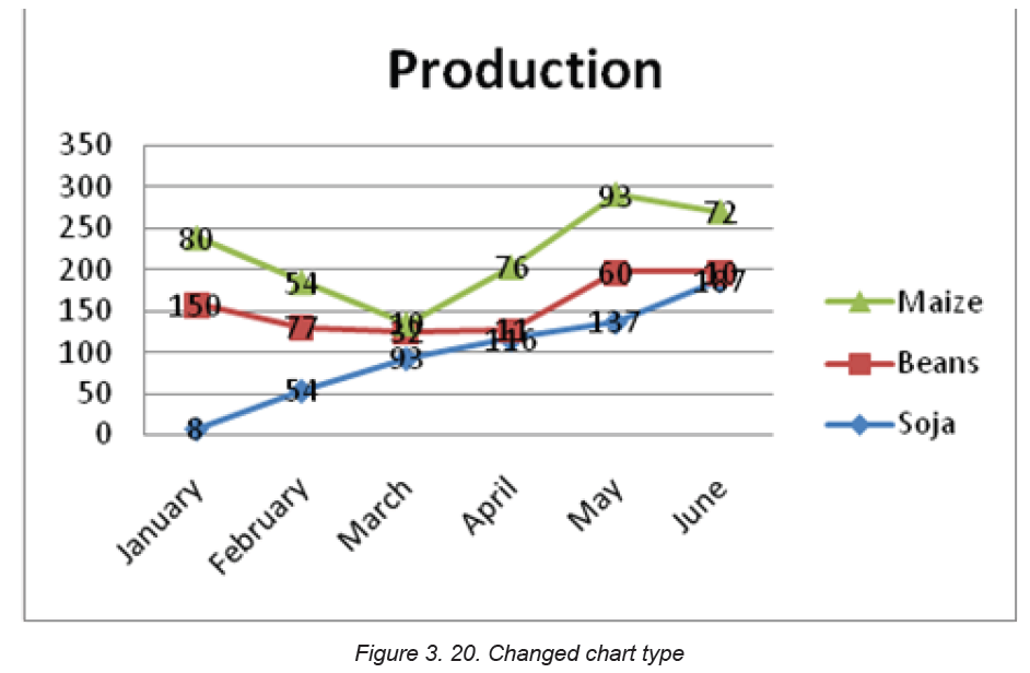
Open the file “Burera Ltd. sales data and do the following:
1. Create a bar column using Burera Ltd. Sales Data2. You have the graph below. Change it to another type (Column chart)
3.3. Data organization
Activity 3.31. Open Burera Ltd Sales data file and update the table as follow:
a. Show salesperson whose region is “Northern”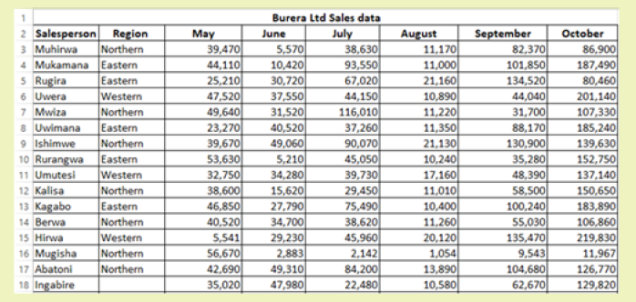
b. Show all salesperson whose sales are below the average
After data has been entered into an Excel worksheet and even after it has
been organized into a table, it can still be manipulated and reorganized. One
of the easiest options is to sort data in a particular order for example, sorting
data in alphabetical order.
On the other hand, Filtering data allows to analyze data easily. When data is
filtered, only rows that meet the filter criteria is going to be displayed and other
rows will be hidden. Filters narrow down the data in a worksheet, allowing to view
only needed information.
3.3.1 Filtering data
After entering data in Excel, it is also possible to filter, or hide some parts of the
data, based on user-indicated categories. When using the Filter option, no
data is lost; it is just hidden from view.
In order for filtering to work correctly, the worksheet should include a header row
which is used to identify the name of each column and is used for filtering.
Follow these steps for filtering data in an excel table:
Step 1: Select the Data tab, and then click the Filter command. Immediately a dropdown
arrow will appear in the header cell for each column. The filter command can
also be accessed by clicking the Home tab and finding it at the far right side of themenu in the Editing Group.
Step 2: Click the drop-down arrow for the column to filter. In this activity column B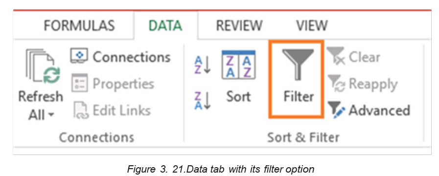
(Region) is filtered to view only certain region.
Step 3: In the Filter menu that will appear uncheck the box next to Select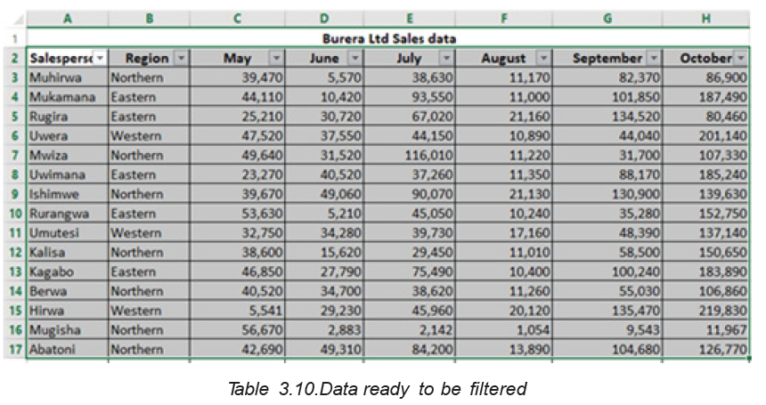
All to quickly deselect all data.
Step 4: Check the boxes next to the data to filter, and then click OK.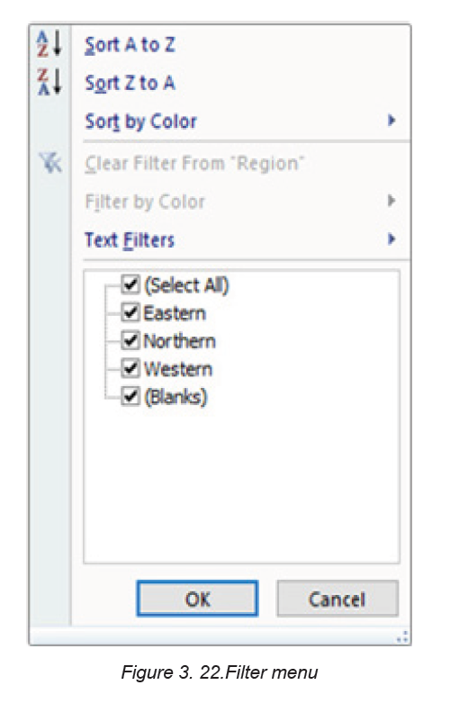
In this example, Northern is checked to view only those types of equipment.
The data will be filtered, temporarily hiding any content that doesn’t match the
criteria.
3.3.2 Clear a filter
After applying a filter, it can be removed or cleared from the worksheet. That
can be in this way:
Step 1: Click the drop-down arrow for the filter that is going to be cleared the
Filter options will appear. In the case of the activity4.3, the column B filter is
going to be cleared.
Step 2: Choose Clear Filter from [COLUMN NAME] from the Filter menu. In
this activity, select Clear Filter from “Checked Out”. This can also be done by
selecting all the items (Northern, Eastern, Western) available in the filter
Step 3: The filter will be cleared from the column. The previously hidden datawill be displayed.
3.3.3. Sorting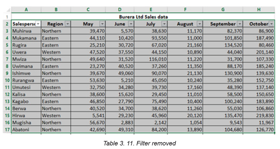
Sorting refers to ordering data in an ascending or descending order according to
some linear relationship among the data items. Sorting can be done on names,
numbers and records.
Below are steps to sort data:
Step 1: Select the entire table to sort. In most cases, select just one cell
and Excel will pick the rest of the data automatically, but this is an error-prone
approach, especially when there are some gaps (blank cells) within the data
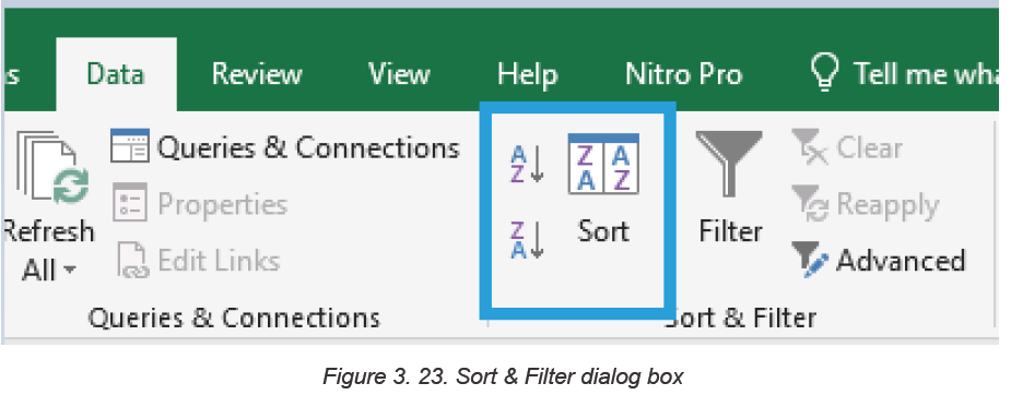
to sort.Step 2: On the Data tab, in the Sort & Filter group, click Sort
Step 3: The Sort dialog box will show up with the first sorting level created
automatically
Note: If the first dropdown is showing column letters instead of headings, tick
off the “My data has headers” box.
Step 4: Click the Add Level button to add the next level and select the options
for another column then click Ok if all needed levels are added. For sorting
by multiple columns with the same criteria, click Copy Level instead of AddLevel. In this case choose a different column in the first box.
After the sorting criteria are applied data will be sorted by Region then by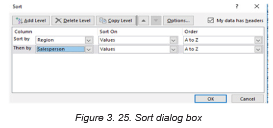
Salesperson as it is clear in the image below:
APPLICATION ACTIVITY 3.3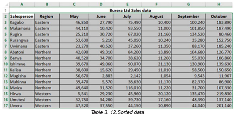
1. Open Burera Ltd Sales data file and update it to make it look likethe table below:
a. Show salespersons whose region is “Western” and sale “Battery”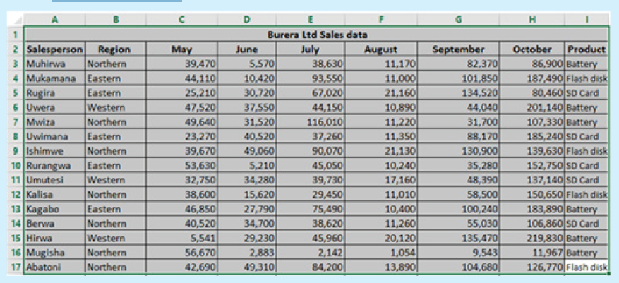
b. as product
c. Sort Product in ascending order by showing the region wherethe product is sold
3.4. Exporting Excel files to PDF or other file types
Activity 3.4
1. Open Burera Ltd Sales data file and export it to a PDF file format
3.4.1 Export Excel Files to PDF
By default, Excel workbooks are saved in the .xlsx file type. However, there may be
times when there is a need to use another file type such as a PDF. Follow the steps
below to export an Excel file to PDF
Step 1:Click on the File menu then Export on bottom of File Menu. A Panel will
appear on right side to Export file in .PDF format. Click on Create PDF/ XPS
Document then on Create PDF/XPS
APPLICATION ACTIVITY 3.3
Open Burera Ltd Sales that you have created in previous activities and do the
following:
1. Export Burera Ltd Sales data File to web page file
2 . Export this same file to PDF. What are the benefits of saving anexcel worksheet to PDF?
Step 2: A Save As window will appear. Select the location where to save the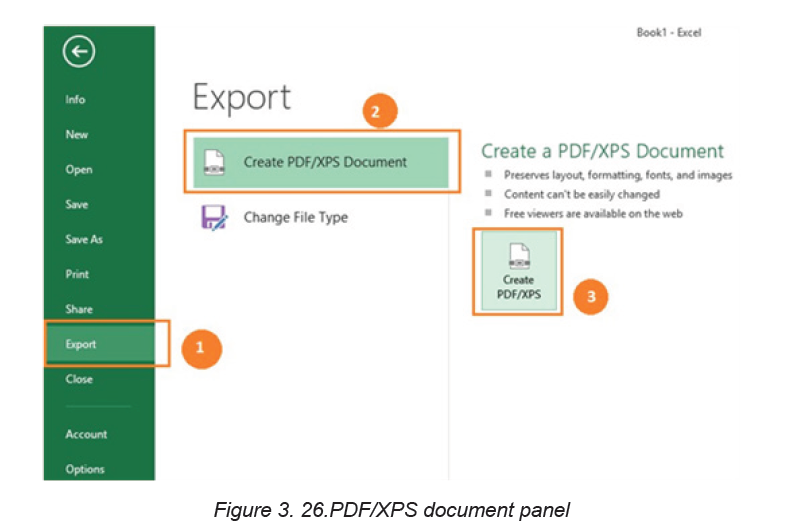
PDF file, give it a name and click Publish.
Excel will Export only the worksheet that is currently active. For exporting to PDF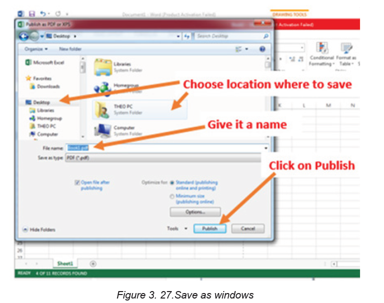
a workbook that has more than one worksheet click on the Option tab available onthe save as window then tick “Entire workbook” and click on OK then on Publish
3.4.2 Exporting in another File Type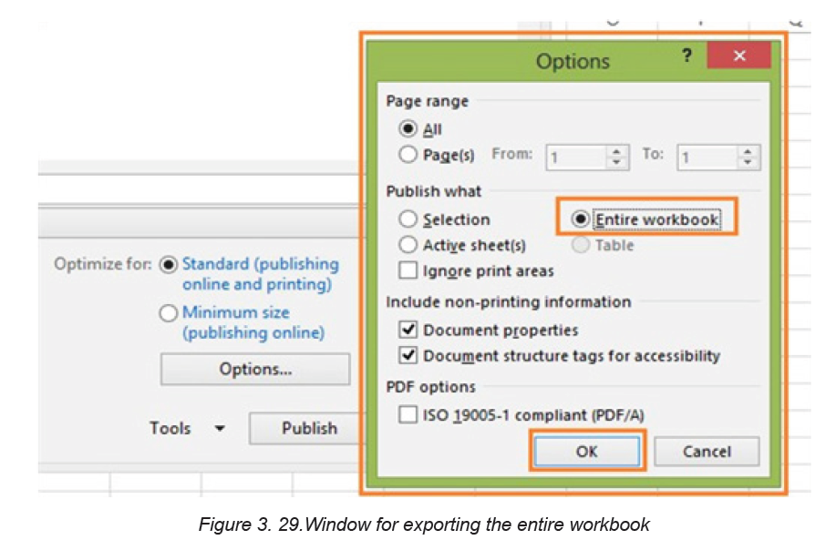
Apart from PDF and other file formats that can be used to save Excel, it is
possible to export an Excel file in other formats like csv, binary workbook and
many others.
To Export Excel files to other formats go through the following steps:.
Step 1:Go to File, then Export. Click on Change File Type and the window belowwith different file types will appear:
Step 2: In the window that will appear choose the new file type to apply and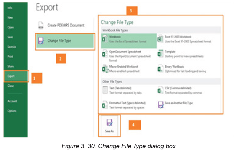
click on Save As in order to provide the name and the location of the file. File
types can be csv, OpenDocument spreadsheet, Macro-Enabled workbook,Text or any other available option.
APPLICATION ACTIVITY 3.4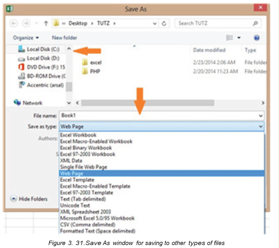
1. Open Burera Ltd Sales that you have created in previous activities and
do the following:
2. Export Burera Ltd Sales data File to web page file
3. Export this same file to PDF. What are the benefits of saving an excel
worksheet to PDF?
End unit assessment
Enter the data below in Excel and save the file under the name “Senior 4 MPCMark Sheet”
1. Calculate the total and the grand total for each student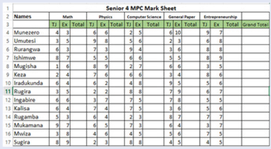
2. Highlight in red and bold students who scored less than 5 points in each
subject
3. Use Green fill with dark green text to Highlight students who have total
above 12 in any subject
4. Using blue highlight show all students who scored 55 and above5. Sort Grand Total in descending order