S4 : Mathematics

 6.0 Introductory activity

2) Go in library or computer lab, do research and make a short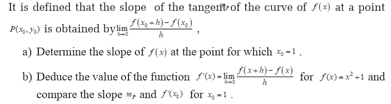 
presentation on the following:
 a. Derivative of a function 

b. Find 2 examples of applications of derivatives.

objectives
 After completing this unit, I will be able to:
 » Use properties of derivatives to differentiate 
polynomial, rational ad irrational functions 
» Use first principles to determine the gradient of the 
tangent line to a curve at a point. 
» Apply the concepts of and techniques of 
differentiation to model, analyze and solve rates or 
optimization problems in different situations. 
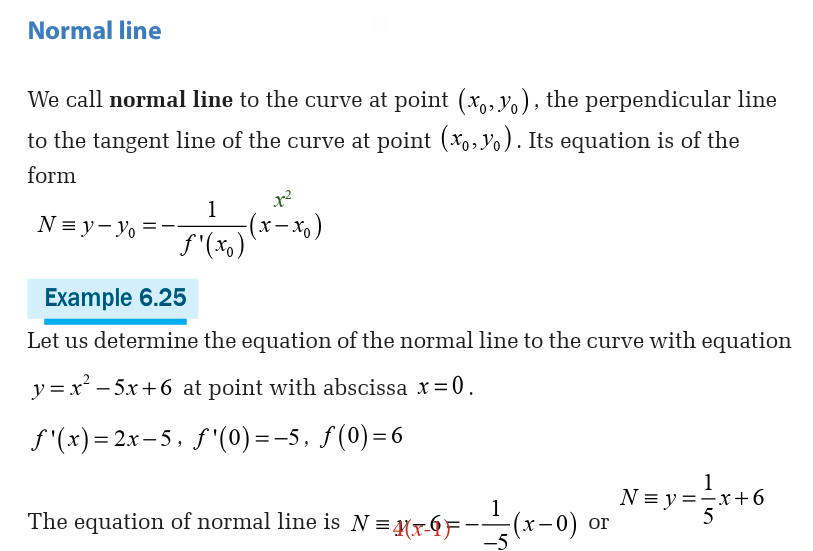
» Use the derivative to find the equation of a line 

tangent or normal to a curve at a given point.

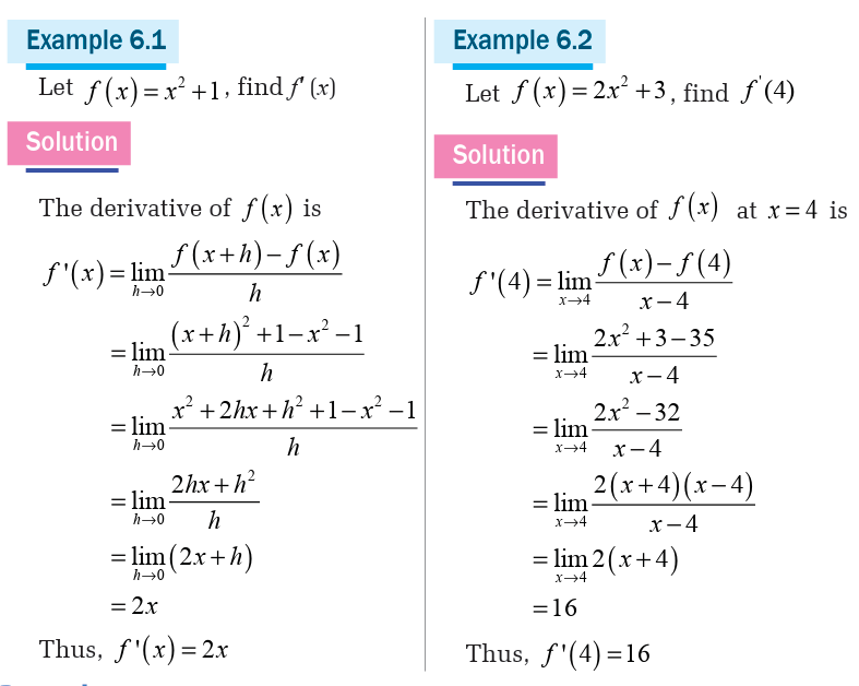
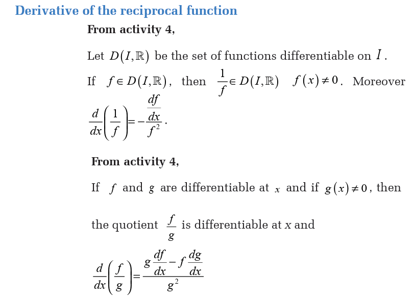
 6.1. Concepts of derivative of a function
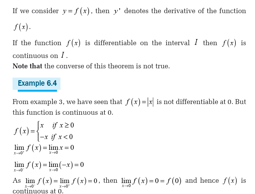
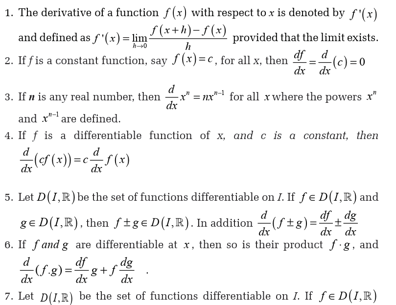
 Definition
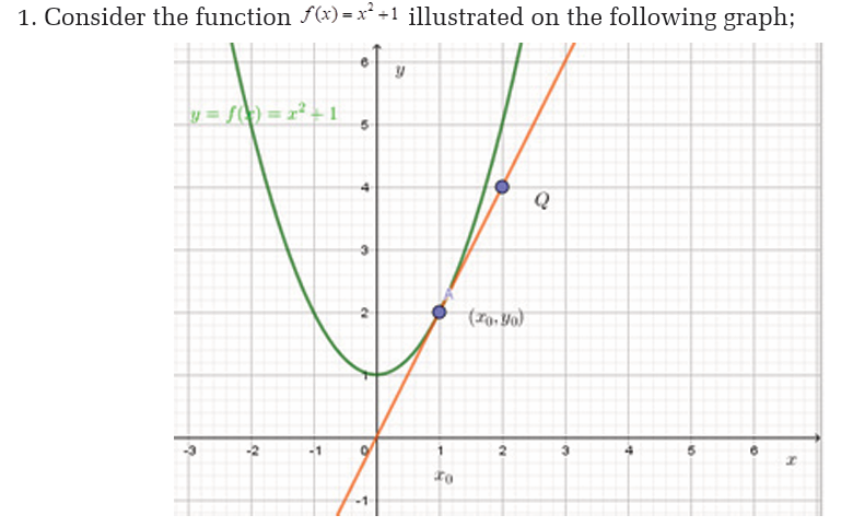
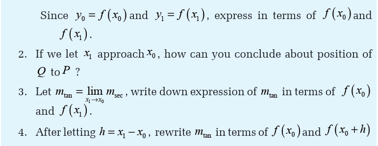
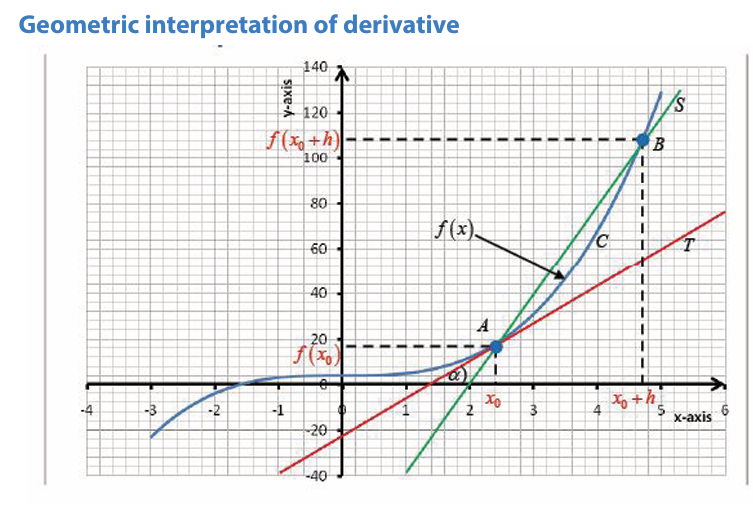
 Activity 6.1.1

 Consider the following figure

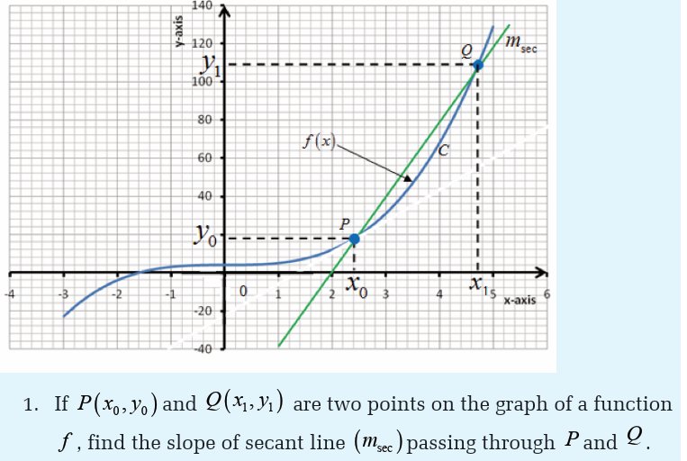
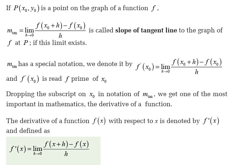
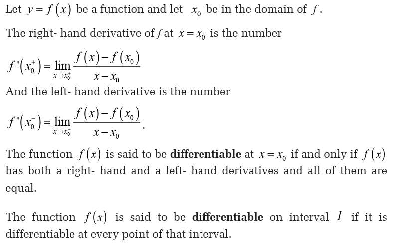
provided that the limit exists.

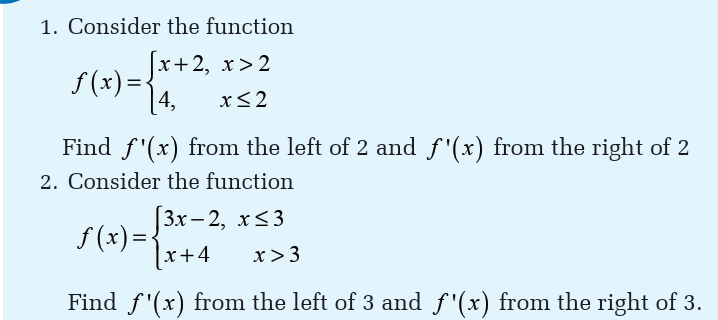
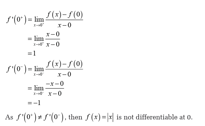
Right-hand and left-hand derivatives

Activity 6.1.2

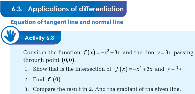
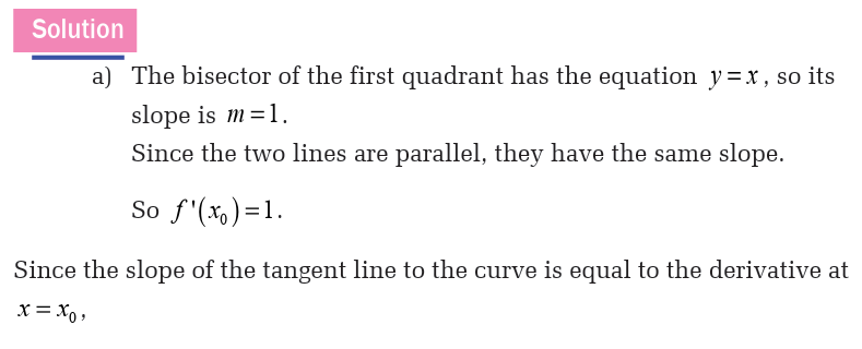
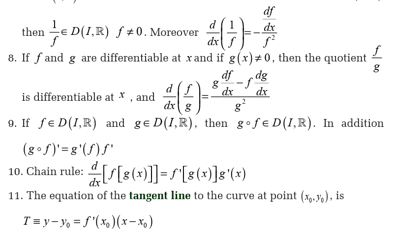
a) Find the point where the tangent line is parallel to the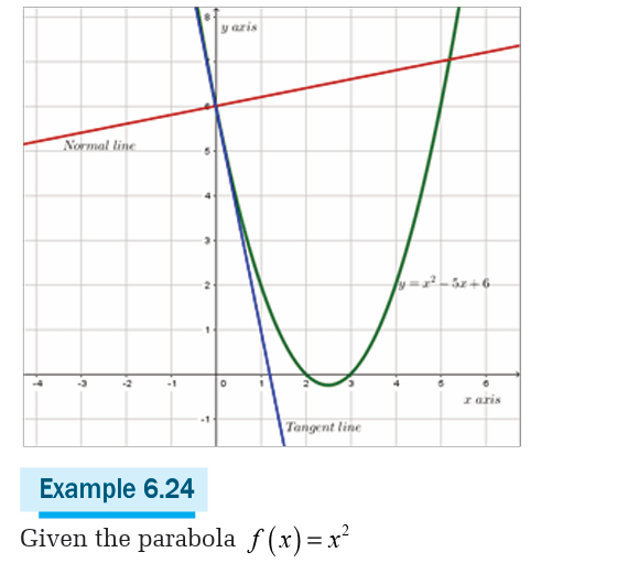 
bisector of the first quadrant. 
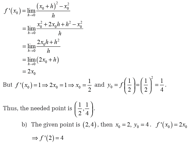
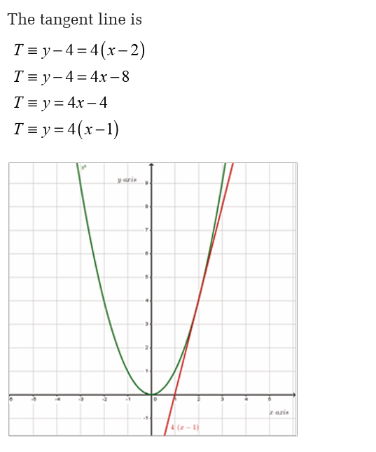
b) Find the tangent line to the curve of this function at point 

(2,4 )

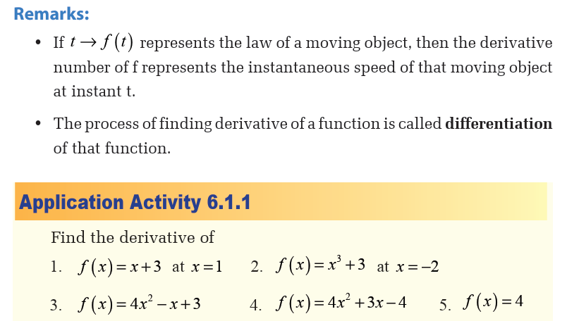
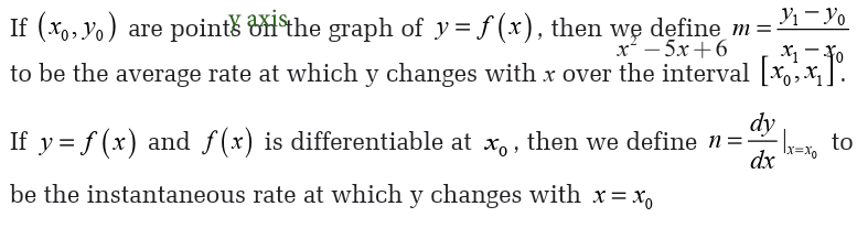
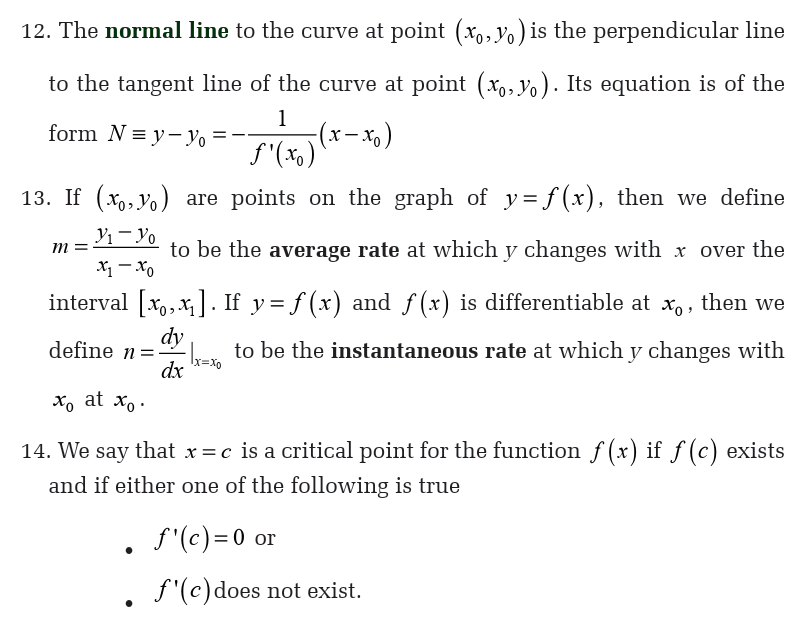
Rates of change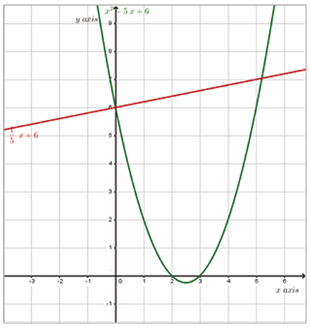
 The purpose here is to remind ourselves one of the more important 
applications of derivatives. That is the fact that represents the rate
of change of 





Now, our derivative is a polynomial and so will exist everywhere. 
Therefore the only critical points will be those values of x which make the 

derivative zero. So, we must solve 

Because this is the factored form of the derivative, it’s pretty easy to identify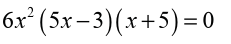

the three critical points. They are,

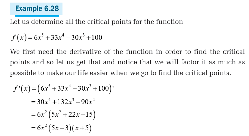
Example 6.29

Let us determine all the critical points for the function

To find the derivative, it’s probably easiest to do a little simplification before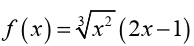 
we actually differentiate. Let’s multiply the root through the parenthesis 
and simplify as much as possible. 
This will allow us to avoid using the product rule when taking the 

derivative.

We will need to be careful with this problem. When faced with a negative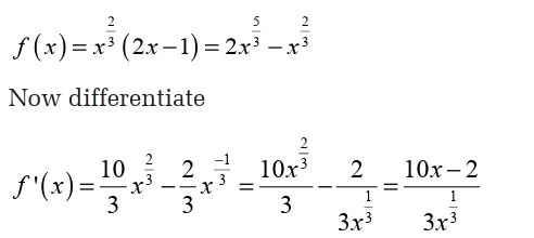 
exponent it is often best to eliminate the minus sign in the exponent as 
we did above. This is not really required but it can make our life easier on 

occasion if we do that.

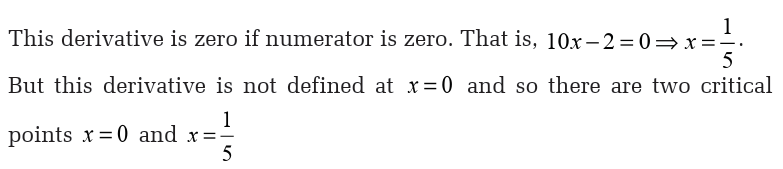
Now, we have two issues to deal with. First the derivative will not exist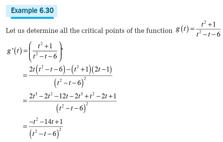 

if there is division by zero in the denominator. So we need to solve, 

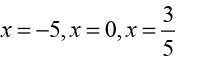
 So, we can see from this that the derivative will not exist at 

However, these are not critical points since the function will also not exist 
at these points. Recall that in order for a point to be a critical point the 
function must actually exist at that point.
 
At this point, we have to be careful. The numerator does not factor, but that 
does not mean that there are not any critical points where the derivative is 
zero. We can use the quadratic formula on the numerator to determine if 

the fraction as a whole is ever zero.

a) Verify that the function is continuous on the interval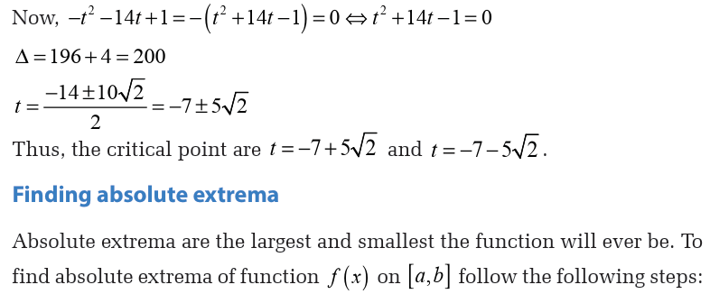 
b) Find all critical points of that are in the interval 
This makes sense if you think about it.  
Since we are only interested in what the function is doing in this 
interval, we do not care about critical points that fall outside the 
interval.
 c) Evaluate the function at the critical points found in a)  above and 
the end points.

 d) Identify the absolute extrema.

It looks like we will have two critical points,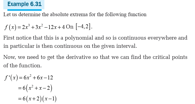 Note that we 
actually want something more than just the critical points. We only want 
the critical points of the function that lie in the interval in question. Both 
of these do fall in the interval as so we will use both of them. 
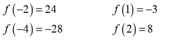
Now we evaluate the function at the critical points and the end points of 

the interval.

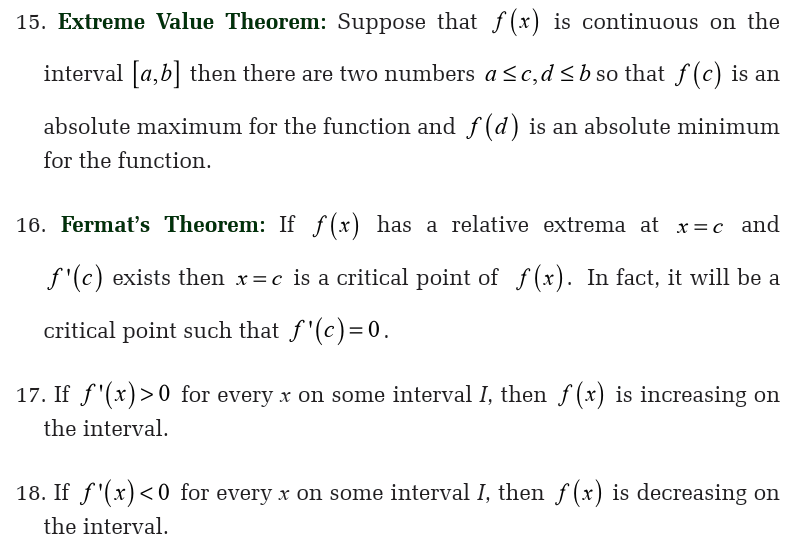
guaranteed to have both an absolute maximum and an absolute minimum 
for the function somewhere in the interval. The theorem doesn’t tell us 
where they will occur or if they will occur more than once, but at least it 
tells us that they do exist somewhere. Sometimes, all that we need to know 
is that they do exist. This theorem doesn’t say anything about absolute 
extrema if we aren’t working on an interval.
 The requirement that a function be continuous is also required in order for 

us to use the theorem. 

 This function is not continuous at x = 0  as we move in towards zero the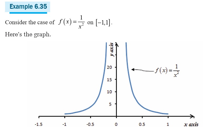 
function is approaching infinity. So, the function does not have an absolute 
maximum. Note that it has an absolute minimum however. In fact the 

absolute minimum occurs twice at both 

If we changed the interval a little to say, 

the function would now have both absolute extrema. We may only run into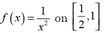 
problems if the interval contains the point of discontinuity. If it doesn’t, 
then the theorem will hold.
We should also point out that just because a function is not continuous at 
a point, that doesn’t mean that it won’t have both absolute extrema in an 

interval that contains that point. 

This graph is not continuous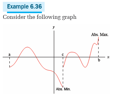  yet it does have both an absolute

maximum  and an absolute minimum 

Also note that, in 
this case one of the absolute extrema occurred at the point of discontinuity, 
but it doesn’t need to. The absolute minimum could just have easily been 
at the other end point or at some other point interior to the region. The 
point here is that this graph is not continuous and yet does have both 
absolute extrema
 The point of all this is that we need to be careful to only use the extreme 
value theorem when the conditions of the theorem are met and not 
misinterpret the results if the conditions are not met. 

Note
 In order to use the extreme value theorem, we must have an interval and the 
function must be continuous on that interval. If we don’t have an interval 
and/or the function isn’t continuous on the interval, then the function may 

or may not have absolute extrema.

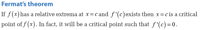
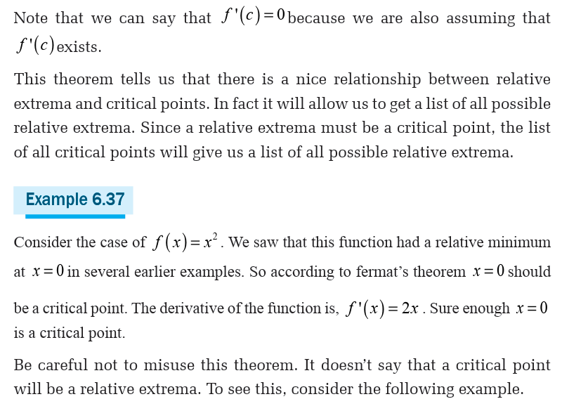
Example 6.38

Clearly  is a critical point.
However this function has no relative 
extrema of any kind. So, critical points do not have to be relative extrema.
 Also note that this theorem says nothing about absolute extrema. An 
absolute extrema may or may not be a critical point.
 
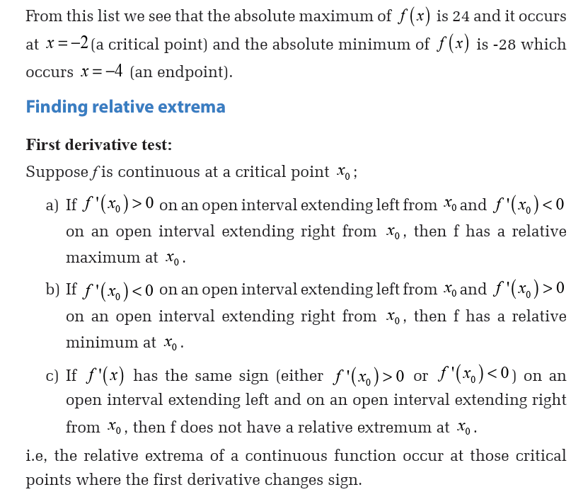
Increasing and decreasing of a function
 In the previous lines we saw how to use the derivative to determine the 
absolute minimum and maximum values of a function. However, there is 
a lot more information about a graph that can be determined from the first 
derivative of a function.The main idea we will be looking at here, we will 
be identifying all the relative extrema of a function. 
We know from our work in previous lines that the first derivative,
is the rate of change of the function. We used this idea to identify where a 

function was increasing, decreasing or not changing. Let us see definitions:

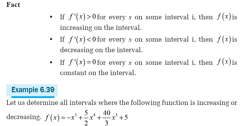
Now, recall that earlier  we constantly used the idea that if the derivative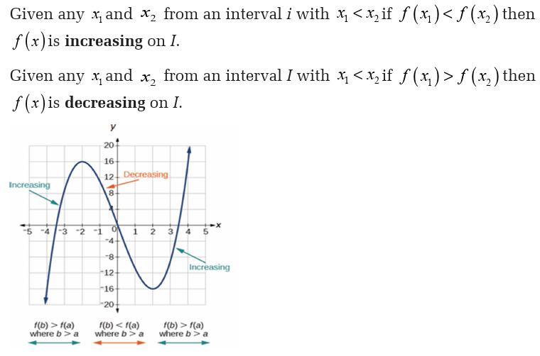 
of a function was positive at a point then the function was increasing at 
that point and if the derivative was negative at a point then the function 
was decreasing at that point. We also used the fact that if the derivative of 
a function was zero at a point then the function was not changing at that 
point. We used these ideas to identify the intervals in which a function is 

increasing and decreasing. This can be summarised in the following fact.

From the factored form of the derivative, we see that we have three critical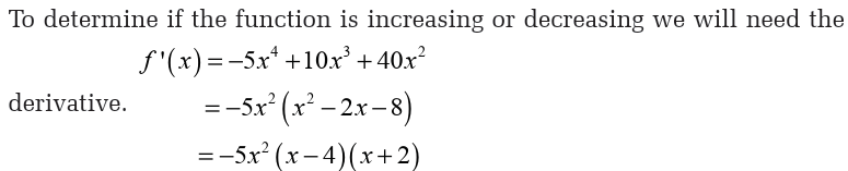
points: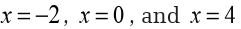We will need these in a bit.
 We now need to determine where the derivative is positive and where it’s 
negative. Since the derivative is a polynomial, it is continuous and so we 
know that the only way for it to change signs is to first go through zero.
 In other words, the only place that the derivative may change signs is at 
the critical points of the function. We have now got another use for critical 
points. So, we will build sign table of graph the critical points 
and pick test points from each region to see if the derivative is positive or 

negative in each region.

Concavity of a function

In the lines, we saw how we could use the first derivative of a function to 
get some information about the graph of a function. In following lines, we 
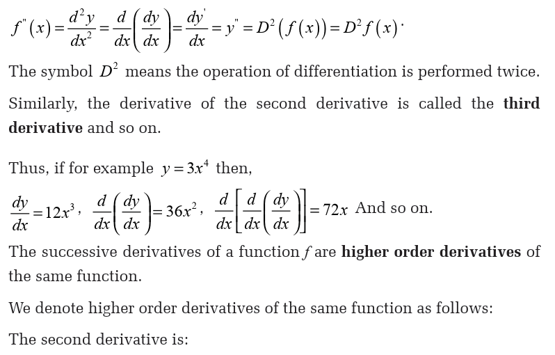
are going to look at the information that the second derivative of a function 

can give us about the graph of a function.

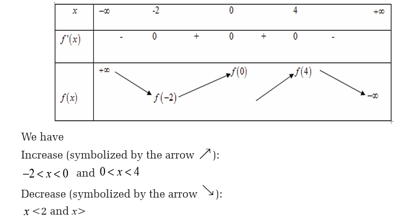
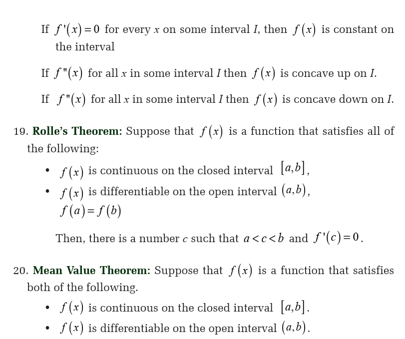
 So a function is concave up if it “opens” up and the function is concave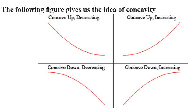 
down if it “opens” down. Notice as well that concavity has nothing to do 
with increasing or decreasing. A function can be concave up and either 
increasing or decreasing. Similarly, a function can be concave down and 

either increasing or decreasing.

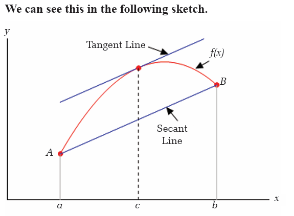
So, as you can see, in the two upper graphs all of the tangent lines sketched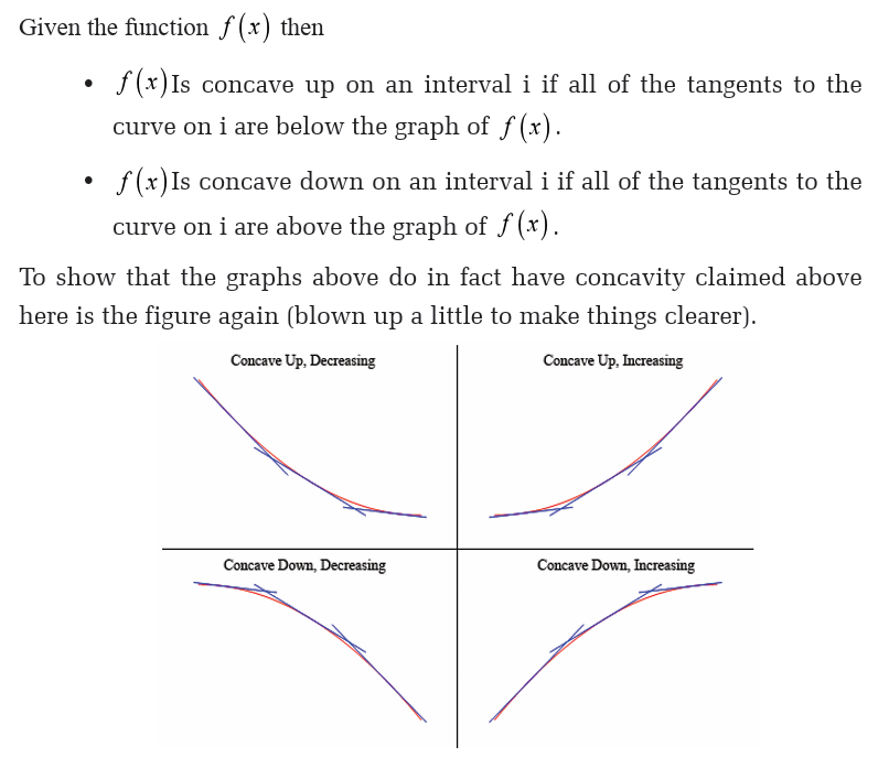 
in are all below the graph of the function and these are concave up. In the 
lower two graphs all the tangent lines are above the graph of the function 

and these are concave down. 

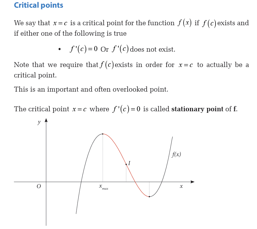
There’s one more definition that we need to get out of the way.
A point  is called an inflection point if the function is continuous at 
the point and the concavity of the graph changes at that point.

Now that we have all the concavity definitions out of the way, we need 
to bring the second derivative into the mix. The following fact relates the 

second derivative of a function to its concavity.

Notice that this fact tells us that a list of possible inflection points will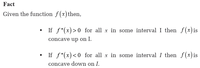 
be those points where the second derivative is zero or doesn’t exist. Be 
careful, however, to not make the assumption that just because the second 
derivative is zero or doesn’t exist that the point will be an inflection point. 
We will only know that it is an inflection point once we determine the 
concavity on both sides of it. It will only be an inflection point if the 

concavity is different on both sides of the point.

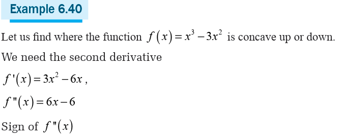
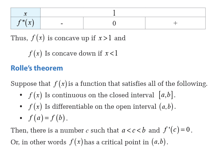
Example 6.42

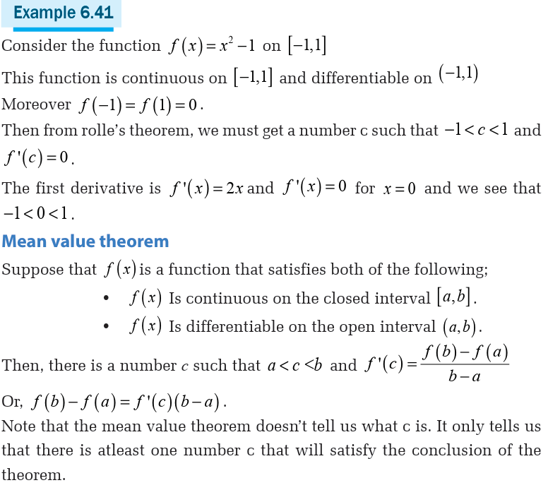
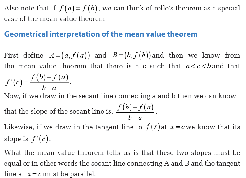
Let us determine all the numbers c which satisfy the conclusions of the mean value

There isn’t really a whole lot to this problem other than to notice that since
 is a polynomial, it is both continuous and differentiable (i.E, the 

derivative exists) on the interval given.

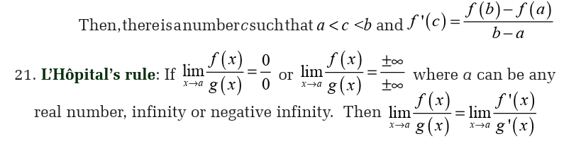
 Now, to find the numbers that satisfy the conclusions of the mean value 
theorem all we need to do is plug this into the formula given by the mean 

value theorem.

 Note that in both of these facts we are assuming the functions are continuous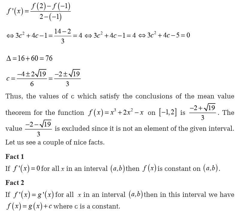 
and differentiable on the interval [ a,b] ,

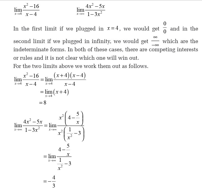
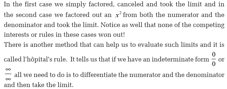
L’hôpital’s rule
 Back on the section of limits, we saw methods for dealing with the following 

limits:

 Applications of differentiation in medicine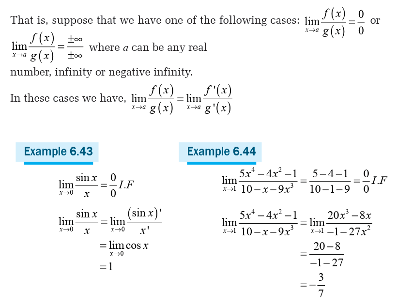
 Application of differentiation to find the Concentration of drugs.
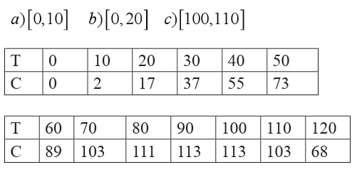
 Example 6.45
 The concentration C (in milligrams per milliliter) of a drug in a patient’s 
blood-stream is monitored over 10minute intervals for 2 hours, where t 
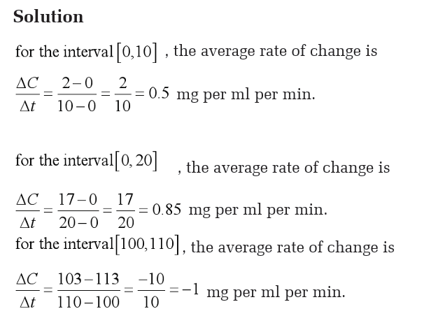
is measured in minutes, as shown in the table. Find the average rate of 

change over each interval.

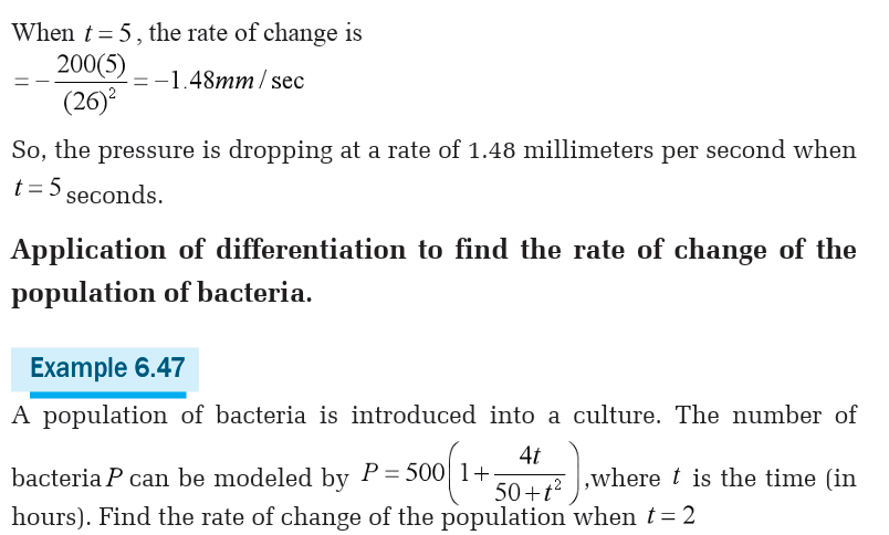
Example 6.46

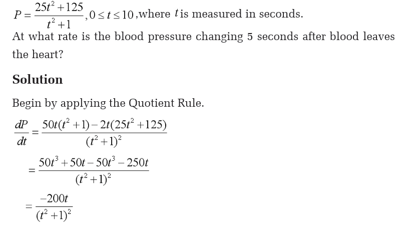
As blood moves from the heart through the major arteries out to the 
capillaries and back through the veins, the systolic blood pressure 
continuously drops. Consider a person whose systolic blood pressure P

(in millimeters of mercury) is given by

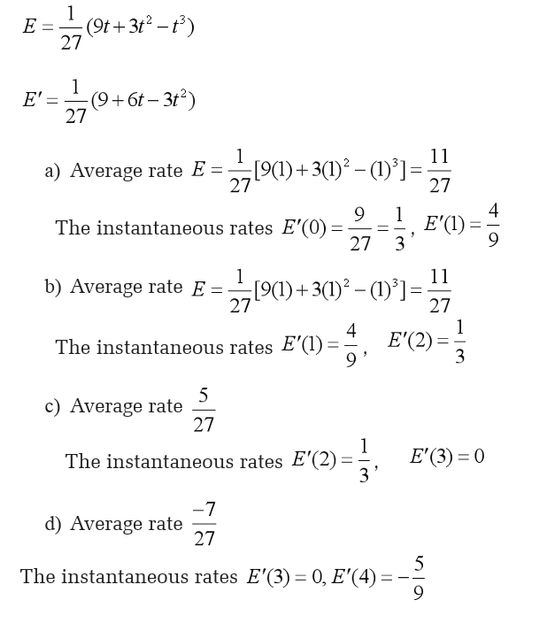
Application of differentiation to find effectiveness E of a pain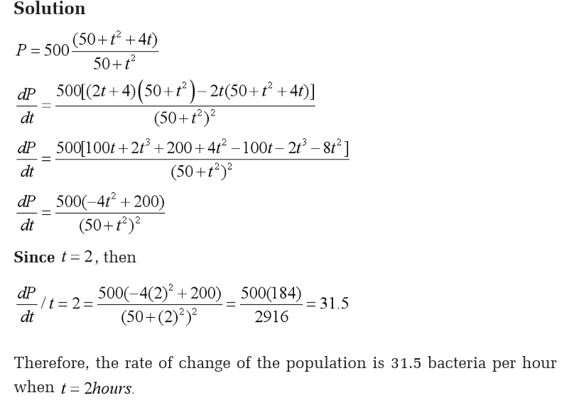
killing drug t hours after entering the bloodstream 
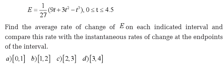
 Example 6.48
 The effectiveness E (on a scale from 0 to 1)  of a pain-killing drug t hours 

after entering the bloodstream is given by.

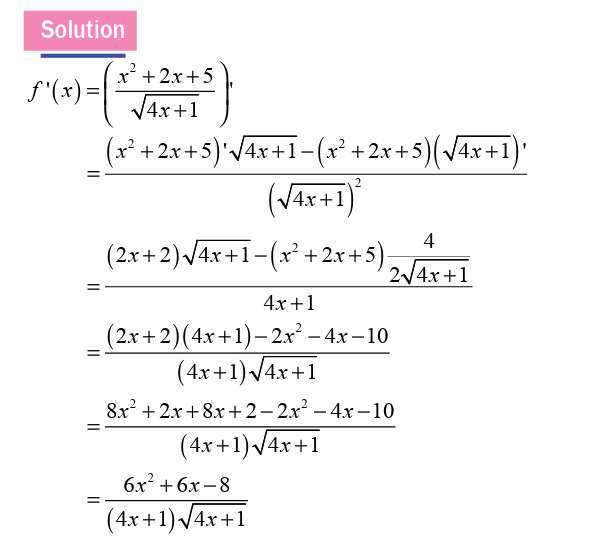
Solution

Unit summary

End Unit Assesment