Content page
Key unit competence
The learner should be able to identify and explain sources of errors in
measurements and report.
My goals
By the end of this unit, I will be able to:
state and explain types of errors in measurements.
distinguish random and systematic errors.
distinguish between precision and accuracy.
explain the concept of significant figures.
explain the error propagation in derived physical quantities.
explain rounding off numbers.
state the fundamental and the derivate quantities and determine
their dimensions.
choose appropriate measuring instruments.
report measured physical quantities accurately.
reduce random and systematic errors while performing experiments.
state correct significant figures of given measurements considering precision required.
Physics for Rwanda Secondary Schools Learner’s Book Senior Two
estimate errors on derived physical quantities.
use dimension analysis to verify equations in physics.
suggest ways to reduce random errors and minimise systematic errors.
Key concepts
1. How does the precision of measurements affect the precision of
scientific calculations?
2. How can one minimise the errors of measurement?
Vocabulary
Accuracy, uncertainty, precision, random, systematic error, rounding off,
significant figures.
Reading strategy
As you read this section, mark paragraphs that contain definitions of key
terms. Use the information you have learnt to write a definition of each key term in your own words.
1.1 Dimensions of physical quantities
1.1.1 Selecting an instrument to use for measuring
Activity 1.1: Selecting a measuring instrument
Suppose we have to measure the following quantities:
⚫ The length and width of classroom.
⚫The thickness of paper.
⚫ The diameter of a wire.
⚫ The length of a football pitch.
⚫ Diameter of a small sphere.
⚫ The mass of a stone
⚫The mass of a feather
Discuss these questions:
1. How would you measure each quantity?
2. What would you use to measure each quantity?
3. Where else would measurements be applied in real life?
In science, measurement is the process of obtaining the magnitude of a
quantity, such as length or mass, relative to a unit of measurement, such
as a meter or a kilogram. The term can also be used to refer to the result
obtained after performing the process.
The different instruments used differ in sensitivity and therefore, we must
always choose one which is most suitable for measuring the quantity
depending on the sensitivity required for the measurement and on the
order of size of the required measurement. The sensitivity of the measuring
instrument is the smallest reading which one can make with certainty using
the instrument. And the accuracy of the readings made on the instrument depends on its sensitivity.
For example, the tape measure is the most suitable instrument for the
measurement of the length of a football field because the order of the
size of the field is within the accuracy which can be obtained from a
tape measure and the tape measure measures up 50m. To measure the
diameter of a wire, you use a micrometer screw gauge because it gives
the accuracy matching the order of the size of the diameter of wire. To
measure the width of a person, a meter rule would be the most suitable judging from the order of the size of a finger.
Note
that each of the instruments has its own advantages and disadvantages
when used. Another important point to note is that we must read the
instruments properly in order to get accurate readings.
Inaccurate
measurements come about if an inaccurate instrument is used or if the
readings are not properly taken from the instrument.
1.1.2 Fundamental and derived physical quantities and their dimension
Physical quantities are divided into two categories, those with dimensions
and those that are dimensionless. Physical quantities with dimensions are classified into Fundamental and derived quantities.
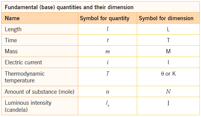
Each of the seven base quantities used in the SI is regarded as having
its own dimension, which is symbolically represented by a single roman capital letter
The symbols used for the base quantities, and the symbols used to denote
their dimension, are given as follows.
Table 1.1: Base quantities and dimensions used in the SI
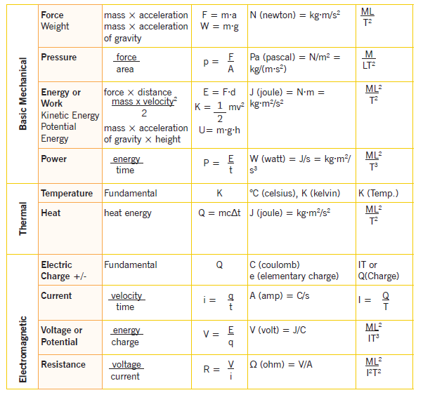
The dimensions of the derived quantities are written as products of powers
of the dimensions of the base quantities using the equations that relate the
derived quantities to the base quantities.
In general the dimension of any quantity Q is written in the form of a
dimensional product, dim Q = LaMbTcTdIeNfJg where the exponents a, b,
c, d, e, and g, which are generally small integers that can be positive,
negative or zero, are called the dimensional exponents.
The dimension of a derived quantity provides the same information about
the relation of that quantity to the base quantities as is provided by the SI
unit of the derived quantity as a product of powers of the SI base units.
There are some derived quantities Q for which the defining equation is such
that all of the dimensional exponents in the expression for the dimension
of Q are zero. This is true, in particular, for any quantity that is defined as
the ratio of two quantities of the same kind. Such quantities are described
as being dimensionless, or alternatively as being of dimension one. The
coherent derived unit for such dimensionless quantities is always the
number one, 1, since it is the ratio of two identical units for two quantities of the same kind.
The unit of a physical quantity and its dimension are related, but not
identical concepts. The units of a physical quantity are defined by convention and related to some standard;
Example:
Length may have units of meters, centimetres, hectometres, millimetres
or micrometers; but any length always has a dimension of L, independent
of what units are arbitrarily chosen to measure it. The physical quantity,
speed, may be measured in units of metres per second; but regardless of
the units used, speed is always a length divided by a time, so we say that
the dimensions of speed are length divided by time, or simply lt. Similarly,
the dimensions of area are L2 since area can always be calculated as a length times a length.
Two different units of the same physical quantity have conversion factors that relate them.
1.1.3 Dimensional analysis
The
fact that an equation must be homogenous enables predictions to be made
about the way in which physical quantities are related to each other.
Examples of the method are given in the table below:
Table 1.2: Dimensional analysis

1.2 Sources of errors in measurement of physical quantities
Activity 1.2: Investigating sources of errors
Take the case of measuring the length and width of an A4 paper.
Material:
⚫A4 paper
⚫ Ruler
Procedure:
Measure the dimensions (width and length) of the given paper using the ruler and record your results.
Discovery:
1. Compare your results with those of other learners.
2. Why are your results different?
3. What would you call those differences?
4. Discuss and explain in pairs your results.
A measurement is an observation that has a numerical value and unit.
When you measure an object, you compare it with a standard unit. Every
measurement must be expressed by a number and a unit. The Oxford
Dictionary explains the term measure as: “Estimate the size, amount or
degree of (something) by using an instrument or device marked in standard
units or by comparing it with an object of known size”.
In order for a measurement to be useful, a standard measurement must
be used.
Standard measurement is an exact quantity that people agree on to be
used for comparison or as a reference to measure other quantities. We
have three kinds of standards: International standard, Regional standard
and National standard.
The science of measurement is called metrology. It has three branches to
know: Legal metrology, Industrial metrology and Material testing.
1.2.1 Types of errors
Activity 1.3: Investigating types of errors
Materials:
⚫Tape measure
⚫Table
Procedure:
⚫Using the tape-measure, measure the length of your table and record the result.
⚫Repeat the same measurement several times and record the results.
⚫Compare your findings.
Questions:
1. Are your results the same?
2. (If not) What may have caused the differences?
3. Where do you think errors come from?
Experimental errors are inevitable. In absolutely every scientific
measurement there is a degree of uncertainty we usually cannot eliminate.
Understanding errors and their implications is the only key to correctly
estimating and minimising them.
The experimental error can be defined as: “the difference between the
observed value and the true value” (Merriam-Webster Dictionary).
The uncertainties in the measurement of a physical quantity (errors) in
experimental science can be separated into two categories: random and
systematic.
⚫Random errors
Random errors fluctuate from one measurement to another. They may
be due to: poor instrument sensitivity, random noise, random external
disturbances, and statistical fluctuations (due to data sampling or
counting).
A random error arises in any measurement, usually when the observer
has to estimate the last figure possibly with an instrument that lacks
sensitivity. Random errors are small for a good experimenter and taking
the mean of a number of separate measurements reduces them in all
cases.
⚫Systematic errors
Systematic errors usually shift measurements in a systematic way.
They are not necessarily built into instruments. Systematic errors can
be at least minimised by instrument calibration and appropriate use of equipment.
A systematic error may be due to an incorrectly calibrated instrument,
for
example a ruler or an ammeter. Repeating the measurement does not
reduce or eliminate the error and the existence of the error may not be
detected until the final result is calculated and checked, say
by a different experimental method. If the systematic error is small a measurement is accurate.
If
you do the same thing wrong each time you make the measurement, your
measurement will differ systematically (that is, in the same direction
each time) from the correct result.
There are two main causes of error: human and instrument.
⚫Human
error can be due to mistakes (misreading 22.5cm as 23.0cm) or random
differences (the same person getting slightly different readings of the
same measurement on different occasions).
For example:
⚪ the
experimenter might consistently read an instrument incorrectly, or might
let knowledge of the expected value of a result influence the
measurements (Bias of the experimenter)
⚪ incorrect measuring
technique: For example, one might make an incorrect scale reading
because of parallax error (reading a scale at an angle)
⚪ failure to interpret the printed scale correctly.
⚫ Instrument errors
can be systematic and predictable (a clock running fast or a metal
ruler getting longer with a rise in temperature). The judgment of
uncertainty in a measurement is called the absolute
uncertainty, or sometimes the raw error. For example:
⚪ errors in the calibration of the measuring instruments.
⚪ zero error (the pointer does not read exactly zero when no measurement is being made).
⚪
the instrument is wrongly adjusted. Although random errors can be
handled more or less routinely, there is no prescribed way to find
systematic errors. One must simply sit down and think about all of the
possible sources of error in a given measurement, and then do small
experiments to see if these sources
are active. The goal of a good
experiment is to reduce the systematic errors to a value smaller than
the random errors. For example a meter stick should have been
manufactured such that the millimeter markings are located much more
accurately than one millimeter.
1.2.2 Accuracy and Precision
The terms accuracy and precision
are often misused. Experimental precision means the degree of exactness
of the experiment or how well the result has been obtained. Precision
does not make reference to the true value; it is just a quality
attribute to the repeatability or reproducibility of the measurement.
Accuracy refers to correctness and means how close the result is to the
true value. Accuracy depends on how well the systematic errors are
compensated. Precision depends on how well random errors are
reduced.
Accuracy is the degree of veracity (“how close to true”) while precision is
the degree of reproducibility (“how close to exact”).
Accuracy
and precision must be taken into account simultaneously. All
measurements have a degree of uncertainty: no measurement can be
perfect!
Precision is to 1/2 of the granularity of the
instrument’s measurement capability. Precision is limited to the number
of significant digits of measuring capability. The precision of a
measurement system, also
called reproducibility or repeatability, is
the degree to which repeated measurements under unchanged conditions
show the same results (degree of exactness).
Accuracy is the degree of closeness between a measured value and a true
value. Accuracy might be determined by making multiple measurements
of the same thing with the same instrument, and then calculating the
average for example, a five kilogramme weight could be measured on a
scale and then the difference between five kilogrammes and the measured
weight could be the accuracy. An accuracy of 100% means that the
measured values are exactly the same as the given values.
A measurement system can be accurate but not precise, precise but
not accurate, neither, or both. For example, if an experiment contains
a systematic error, then increasing the sample size generally increases
precision but does not improve accuracy. Eliminating the systematic error
improves accuracy but does not change precision.

Fig. 1.1: Accuracy and precision
A measurement system is called valid if it is both accurate and precise.
Uncertainty depends on both the accuracy and precision of the
measurement instrument. The lower the accuracy and precision of
an instrument, the larger the measurement uncertainty is. Often, the
uncertainty of a measurement is found by repeating the measurement
enough times to get a good estimate of the standard deviation of the values.
Physical measurements are never exact but approximate because of
error associated with the instruments (limitations of the measuring
instrument) or which arise when using them (the conditions under which
the measurement is made, and the different ways the operator uses the
instrument). For example, it is possible to have readings taken with great
precision which are not accurate i.e. using an inaccurate instrument of
high sensitivity (precision). For example, if the instrument being used has
a zero error which has not been taken care of, the measurements read
from it are consistently affected by the zero error. Similarly, it is possible to
have readings which are accurate but not very precise. This occurs if one
uses an accurate instrument of low sensitivity (precision).
Example of measurement using a ruler
⚫ Using a ruler with 0.5cm marking, we might measure this eraser to be 5.5cm long.
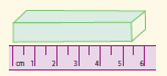
⚫ I f we used a more precise ruler, with 0.1cm markings, then we find the length to be 5.4cm.
⚫ I f we used a micrometer that measured to the nearest 0.01cm,
we may find that the measured length is 5.41cm.
The Limit of Accuracy of a Measuring Instrument are ± 0.5 of
the unit shown on the instrument’s scale. It is important to assess
the uncertainty in measurements. One way to do this is to repeat
measurements and average the results. The maximum deviation
from the average is one way to assess uncertainty (although not
the best way). In the following measurements, measure each case
at least three times and take an average. Then record the number
like the following example: Measured times: 5.6s, 6.0s, 6.2s; Average: 5.9s
Experimental time: ![]()
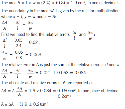
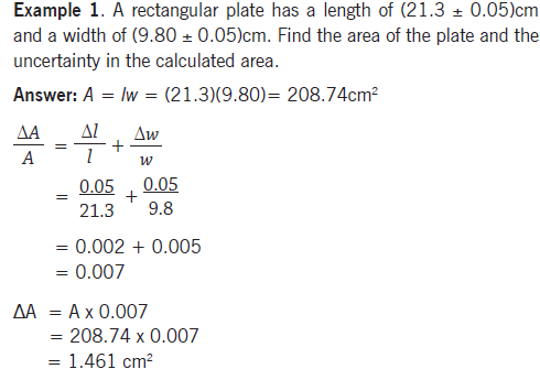
1.2.3 Calculations of errors
When combining measurements in a calculation, the uncertainty in the
final result is larger than the uncertainty in the individual measurements.
This is called propagation of uncertainty and is one of the challenges of
experimental physics. As a calculation becomes more complicated, there
is increased propagation of uncertainty and the uncertainty in the value of
the final result can grow to be quite large.
There are simple rules that can provide a reasonable estimate of the
uncertainty in a calculated result:
1. Absolute and Relative Errors (Uncertainties)
When reading a scale it is standard practice to allow an error of one
half of a scale division (depending on the scale being used and the
operator’s eyesight). But as well as the reading being judged there
is also the zero setting to be judged and this also has an uncertainty
of half of a scale division. So for most instruments the total error for
a measurement is ![]() 1 scale division.
1 scale division.
The case (i), is referred to as the absolute error, the Case (ii), as the
relative error (which is often expressed as a percentage). In some
other cases it is easier to work with absolute rather than relative errors (and vice-versa), so be familiar with both.
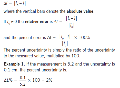

In experimental measurements, the uncertainty in a measurement
value is not specified explicitly. In such cases, the uncertainty is
generally estimated to be half units of the last digit specified. For
example, if a length is given as 5.2cm, the uncertainty is estimated to be 0.5mm.
• Operations with errors
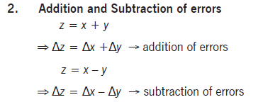
When measurements with uncertainties are added or subtracted, add
the
absolute uncertainties of either addition or substraction errors in
order to obtain the absolute uncertainty of the measurement.
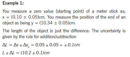

Activity 1.4: Length measurement of a stick
Measure a zero value (starting point) of a meter stick as xo.
Measure the position of the end of the given stick as being x.
Question:
Find the length of that stick.
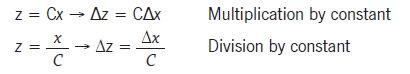
3. Multiplication and Division
Multiplication and Division by a constant

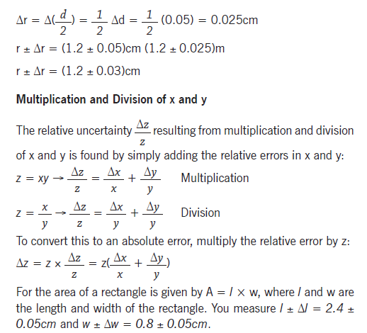
We round the absolute uncertainty to 1 sig fig and match precisions
in our final answer; the relative uncertainty is rounded to the same
sig figs as the answer in the absolute case.


We round the absolute uncertainty to 1 sig fig and match precisions
in our final answer; the relative uncertainty is rounded to the same
sig figs as the answer in the absolute case.
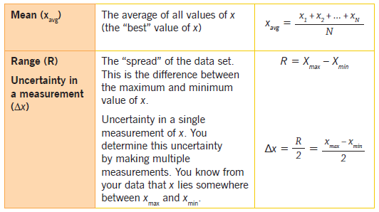
1.3 Estimating the uncertainty range of measurement
Repeated measurements allow you to not only obtain a better idea of
the actual value, but also enable you to characterise the uncertainty of
your measurement. Below are a number of quantities that are very useful
in data analysis. The value obtained from a particular measurement is
repeated N times. Often times in lab N is small, usually no more than 5 to
10. In this case we use the formulae below:
Table 1. 3: Uncertainty calculation
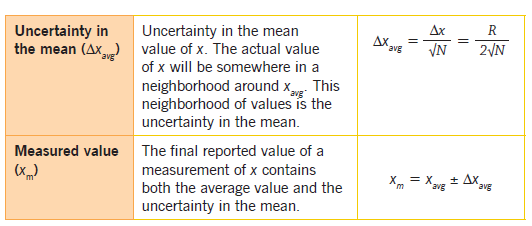
The average value becomes more and more precise as the number of
measurements N increases. Although the uncertainty of any single
measurement is always, the uncertainty in the mean, it becomes smaller
(by a factor of ) as more measurements are made.
Example:
You measure the length of an object five times.
You perform these measurements twice and obtain the two data sets
below.
Table 1. 4: Measurement data
Given the table below, use these measurements recorded in the two data
sets and calculate the mean, the range, the uncertainty measurement, the
uncertainty in the mean and the measured value.
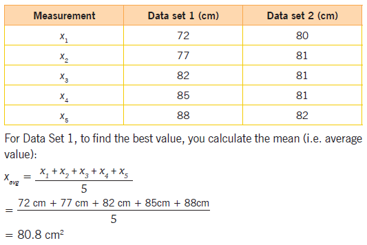
The range, uncertainty and uncertainty in the mean for Data Set 1 are
then:

![]()
For Data Set 2 yields the same average but has a much smaller range. Form
groups of 4 to reproduce the average mean, the range, the uncertainty,
uncertainty in measurement and the reported measured length.
1.4 Significant figures of measurements
No quantity can be measured exactly. All measurements are approximations.
A digit that was actually measured is called a significant digit. Significant
digits may be shown on measuring devices (rulers, meters, etc.) as tick
marks or displayed digits, although you can’t always be sure. The number of
significant digits is called precision. It tells us how precise a measurement
is— how close to exact. For example if you say that the length of an object
is 0.428 m, you imply an uncertainty of about 0.001m.
If a quantity is written properly, all the digits are significant except place
holding zeroes.
The significant figures (also called significant digits and abbreviated sig
figs, sign. figs or sig digs) of a number are those digits that carry meaning
contributing to its precision. Significant figures in a measurement are the
digits in the measurement which are obtained from the instrument with
certainty together with the first digit which is uncertain (estimate).
1.4.1 The rules for identifying significant digits
The rules for identifying significant digits when writing or interpreting
numbers are as follows:
⚫ All non-zero digits are considered significant. For example, 91 has
two significant figures (9 and 1), while 123.45 has five significant
figures (1, 2, 3, 4 and 5).
⚫ Zeros appearing anywhere between two non-zero digits (trapped
zeroes) are significant. Example: 101.12 has five significant
figures: 1, 0, 1, 1 and 2.
⚫ Leading zeros (zeroes that precede all non-zero digits) are not
significant. For example, 0.00052 has two significant figures: 5
and 2. Leading zeroes are always placeholders (never significant).
For example, the three zeroes in the quantity 0.002 m are just
placeholders to show where the decimal point goes. They were
not measured. We could write this length as 2 mm and the zeroes
would disappear.
⚫ Trailing zeros (zeros that are at the right end of a number) in a
number containing a decimal point are significant. For example,
12.2300 has six significant figures: 1, 2, 2, 3, 0 and 0. The number
0.000122300 still has only six significant figures (the zeros before
the 1 are not significant). In addition, 120.00 has five significant
figures. This convention clarifies the precision of such numbers;
for example, if a result accurate to four decimal places is given as
12.23 then it might be understood that only two decimal places
of accuracy are available. Stating the result as 12.2300 makes it
clear that it is accurate to four decimal places.
⚫ The significance of trailing zeros in a number not containing a
decimal point can be ambiguous. For example, it may not always
be clear if a number like 1300 is accurate to the nearest unit (and
just happens coincidentally to be an exact multiple of a hundred)
or if it is only shown to the nearest hundred due to rounding or
uncertainty. Various conventions exist to address this issue:
⚪
A bar may be placed over the last significant digit; any trailing zeros
following this are insignificant. For example, has three significant
figures (and hence indicates that the number is accurate to the nearest
ten).
⚪ The last significant figure of a number may be underlined; for example, “20000” has two significant figures.
⚪ A decimal point may be placed after the number; for example
“100.” indicates specifically that three significant figures are meant.
Generally, the same rules apply to numbers expressed in scientific
notation. For example, 0.00012 (two significant figures) becomes
1.2×10⁻⁴, and 0.000122300 (six significant figures) becomes
1.22300×10⁻⁴.
In particular, the potential ambiguity about the significance of trailing
zeros is eliminated. For example, 1300 to four significant figures is
written as 1.300×10³, while 1300 to two significant figures is written
as 1.3×10 3.
Numbers are often rounded off to make them easier to read. It’s easier
for someone to compare (say) 18% to 36% than to compare 18.148% to
35.922%.
Note:
Zeros at the end of a number but to the left of a decimal, in
this handbook will be treated as not significant for example
1 000 m may contain from one to four significant figures,
depending on precision of the measurement, but in this hand
book it will be assumed that measurements like this have one
significant figure.
⚫ Do not confuse significant figures with decimal places. For
example, consider measurements yielding 2.46 s, 24.6 s
and 0.002 46 s. These have two, one, and five decimal
places, but all have three significant figures.
⚫ If a number is written with no decimal point, assume
infinite accuracy; for example, 12 means 12.0000….
1.4.2 Special rules of calculation with significant figures
The final answer should not be more precise than the least precise
measurement in your data. For example, though your calculator gives an
answer to nine digits, do not give this number of digits in your final answer.
Example: Perform these calculations, following the rules for significant
figures
1. Addition or subtraction: the final answer should have the same
number of digits to the right of the decimal as the measurement
with the smallest number of digits to the right of the decimal.
![]()
( ≅Means, approximately equal to)
2. Multiplication or division: the final answer has the same number
of figures as the measurement having the smallest number of
significant figures.
123 × 5.35 = 658.05 = 658
11.2 × 6.8 = 77 (6.8 has the least number of significant figures,
namely two)
2035cm × 12.5m = 20.35m × 12.5m =254.375m2 = 2.54 ×
104 cm2 (it is better to make the conversion to the same units before
doing any more arithmetic)
1.5 Rounding off numbers
Activity 1.5: Rounding off a number
Using your ruler; measure the width (w) of a note book seven times
and perform the average as:
Questions:
• Round off your result to 2 decimal places
The concept of significant figures is often used in connection with rounding.
For example, the population of a city might only be known to the nearest
thousand and be stated as 52,000, while the population of a country
might only be known to the nearest million and be stated as 52,000,000.
When we compute with measured figures, we often round off numbers so
that they will show the precision or accuracy that is appropriate.
In rounding off, we drop digits or replace digits with zeros to make numerals
easier
to use and interpret. Instead of saying 45,125 people attended the
football match last Sunday; we would probably round the value to 45,000
people. When we replace digits with zeros by rounding off, the
zeros
are not significant. In rounding off a number, the digits dropped must
be replaced by ‘place holding’ zeros. The following rules will be found
useful when rounding off figures:
⚫ If the first of the digits to
be dropped (reading from left to right) is 1, 2, 3 or 4, simply replace
all dropped digits with the appropriate number of zeros. For example,
57,384 rounded off to the nearest
thousands becomes 57,000.
⚫ If
the first of the digits to be dropped (reading from left to right) is 6,
7, 8 or 9, increase the preceding digit by 1. For e.g., 5,383 rounded
off to the nearest hundred becomes 5,400.
⚫ If only one digit is to
be dropped and this digit is 5, increase the preceding digit by 1 if it
is odd, and leave it unchanged if it is even. Thus, if 685 is to be
rounded off to the nearest tens it becomes 680, while 635 rounded off to
the nearest tens becomes 640.
⚫ If a decimal fraction is rounded
off, zeros should not replace the digits that are to the right of the
decimal, because zeros to the right of a decimal are significant. For
example, 73.2 rounded off to one
significant figure becomes 70 and not 70.0 to the nearest tens.
1.6 Unit 1 assessment
1. The learners listed below measured the density of a piece of lead
three times. The density of lead is actually 11.34 g/cm3. Below
are their results;
a) Rachel: 11.32 g/cm3, 11.35 g/cm3, 11.33 g/cm3
b) Daniel: 11.43 g/cm3, 11.44 g/cm3, 11.42 g/cm3
c) Leah: 11.55 g/cm3, 11.34 g/cm3, 11.04 g/cm3
(i) Whose results were accurate?
(ii) Whose were precise?
(iii) Whose measurements were both accurate and precise?
2. Arrange the following measurements in order of precision beginning with the most precise: 17.04cm; 843 cm; 0.006cm; 342.0cm.
3. Round off to;
a) the nearest unit: 6.8; 10.5; 801.625,
b) the nearest tenth 5.83; 480.625; 0.234; 0.285; 6.58;
36.092,
c) the nearest hundredth: 3.632; 812.097; 0.71
d) the nearest thousandth: 0.2827; 0.0066.
e) the nearest tens: 56; 44; 17; 656,
f) the nearest hundreds: 219; 256; 71,550; 930.7,
g) the nearest thousands: 890; 1600; 10 500; 13 856; 5420.5
4. Round off the following measurement so that all have the same
degree of accuracy: 468.5m; 0.00708m; 3.467m; 56.93m; 3.004m
5. Perform the following operations, rounding off each answer to
the proper degree of accuracy:
a) 6.574 + 34.57 =
b) 23.12 × 34.9 =
c) 5.2 – 5.7 =
d) 625/15 =
e) Sqrt(5625) =
6. Round off the numbers below to the shown number of significant
figures in the brackets:
a) 245 086 (4);
b) 406.50 (3)
c) 8 465 (3);
d) 84.25 (2);

12. If an equation is dimensionally correct, does this mean that
the equation must be true? If an equation is not dimensionally
correct, does this mean that the equation cannot be true?
13. Is it possible to add a vector quantity to a scalar quantity? Explain.
14. If A = B, what can you conclude about the components of A and B?