ICT

Key Unit Competency: By the end of this unit, you should be able to:

1. Work with spreadsheets to apply complex formulas and functions recognising the order of operations. 

2. Apply conditional formatting to the content of a worksheet. 

3. Use absolute and relative referencing. 

Introduction 

Spreadsheets are programmed in such a way that they can accept different formulas and functions.Formulas may comprise a combination of actual values, cell references, functions and mathematical operators. When the correct formula is typed in the formula bar, the result of the formula appears in the active cell.

7.1 Predefined Operators and Symbols in Microsoft Excel

Some predefined operators used in excel include: addition, subtraction, multiplication and division operators which have been discussed in Unit 4. The symbols used include:

 7.2 Complex Formulas

In Unit 4, we discussed how to create simple formula involving a single operator. Excel has a provision of using complex formula. 

They are written using more than one operator. Example of a complex formula is = (B2 + B3)/2 written in cell B5. In this case, the operators used are addition and division. 

Creating Complex Formulas 

The following are the steps followed when creating complex formulas. 

(i) Click the cell where the result of the formula is to be displayed such as B5. 

(ii) Type the equal sign. 

(iii) Type an opening parenthesis. 

(iv) Click on the first cell tobe included in the formula or type the cell address such as B2. 

(v) Type the mathematical operator such as (+). 

(vi) Click on the second cell in the formula or type the cell address such as B3. 

(vii) Type a closing parenthesis. 

(viii) Type the next mathematical operator such as (/).

(ix) Type the next cell address or value such as 2.

(x) Press Enter, or click the Enter button on the Formula bar to end the formula. For example, figure 7.1 on page 188 shows the formula =(B35+B36)/2 entered in cell B38.

Figure 7.1: The formula for computing the average bill for January

7.3 Cell References 

They are also known as cell addresses. Cell address consists of a column letter and row number. They are used in formulas. There are three types of cell references, namely relative, absolute, and mixed cell references. 

(i) Relative cell reference:This type of reference automatically changes the cell addresses of a formula relative to the position of the cell where it is copied.  For example, if the formula =A1+B1+C1 is written in cell D1 then copied to cell F1, the formula becomes =C1+D1+E1. It is the default cell referencing style used in excel anytime a formula is entered.

(ii) Absolute cell reference: In this type of reference, the formula remains the same regardless of where it is copied. To make a cell absolute, type dollar signs before the column letter and the row number.  For example, $A$1 is an absolute cell reference of cell A1. If the formula =($A$1*$B$1) is written in cell C1 then copied to G1, it remains =($A$1*$B$1).

(iii) Mixed cell reference: It is a type of reference that combines both relative and absolute cell reference. To apply this reference, the $ sign appears on the column letter or row number in the cell reference but not on both. The row could be made absolute while the column is relative or vice versa. For example: Table 7.1 shows some examples of cell references together with an explanation of each.

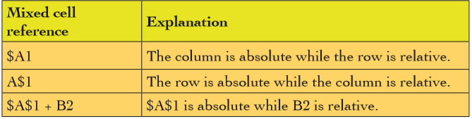
Table 7.1: Mixed cell references and their explanation 

If any of these references are written in cell E2 then copied to cell G2 the formula would become:

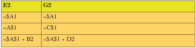 Table 7.2: Example of mixed cell references

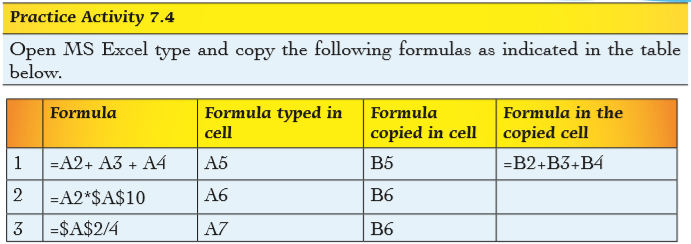
7.4 Cell References of another Worksheet

In Spreadsheets, it is possible to refer to a cell in another worksheet. Information can also be copied from a worksheet then pasted to another. 

7.4.1 Copy Paste Option 

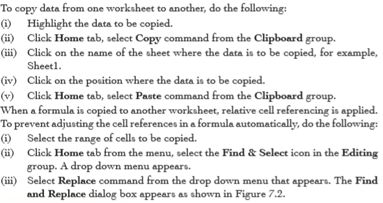
Figure 7.2: Find and replace dialog box

(iv) In the Find What box type “=”, and in the Replace With box type “#”.  

(v) Click Replace All, to replace all occurrence of “=” with “#” in the range then close the dialog box. The formula is changed to a label. For example “=A1*B1” becomes “#A1*B1”. 

(vi) Copy and paste the formula to the desired location in another worksheet. 

(vii) To change it back to formula, simply replace all occurrence “#” with“=”.

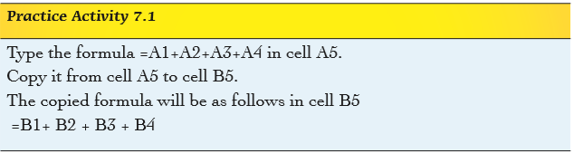
Copying formula 

Once a formula is entered in a cell, it can be copied to other cells within the worksheet. When a formula is copied, the cell references are automatically adjusted depending on the type of reference used in the original formula. To copy a formula, do the following: 

(i) Click on the cell that contains the formula. 

(ii) Move the cursor to the fill handle of the cell selector. Ensure that the cursor changes to a plus sign.

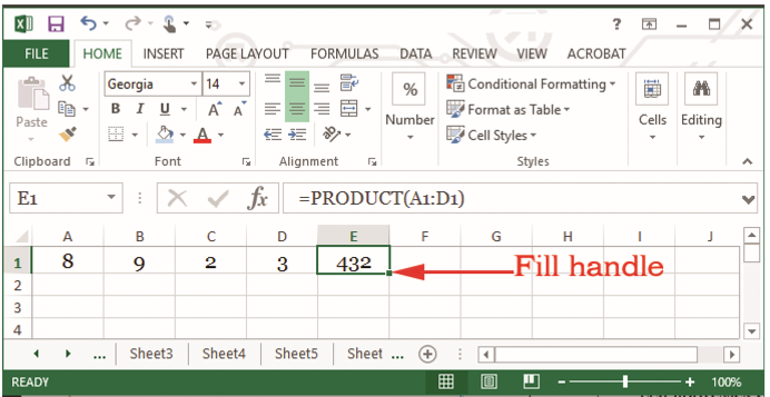
Figure 7.3: Copying a formula to the desired location 

(iii) Click and drag the cursor either across the row or column. Release the button once all the cells where the formula is to be copied are selected. 

Note:The formula can also be copied by right-clicking on it then selecting Copy command from the pop-up menu that appears. Right-click on the cell where the data is to be copied, then select Paste. 

7.4.2 Sheet Reference
  
Instead of the copy paste option, the user can decide to write a formula to reference a specific value from another worksheet. 
 

Alternatively, type the formula by beginning with the equal sign then sheet name then exclamation mark (!) and then the cell reference such as E14, for example, =Sheet1!E14: Sheet1 is the name of the sheet where the data is being obtained from.

Figures 7.5 to 7.9 show different worksheets and the formula when content is copied to a different worksheet.

Figure 7.5: Data entered in Worksheet 1

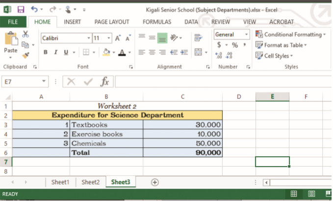
Figure 7.6: Data entered in Worksheet 2

Figure 7.7: Data entered in Worksheet 3

Figure 7.8: Data entered in Worksheet 4

Figure 7.9: Data entered in Worksheet 5 

The Worksheet in figure 7.8 displays the formula used in sheet reference whereas the worksheet in figure 7.9 shows the actual values. The advantage of using sheet referencing is that whenever values in the original sheet are changed, the values are automatically updated in the other worksheets.

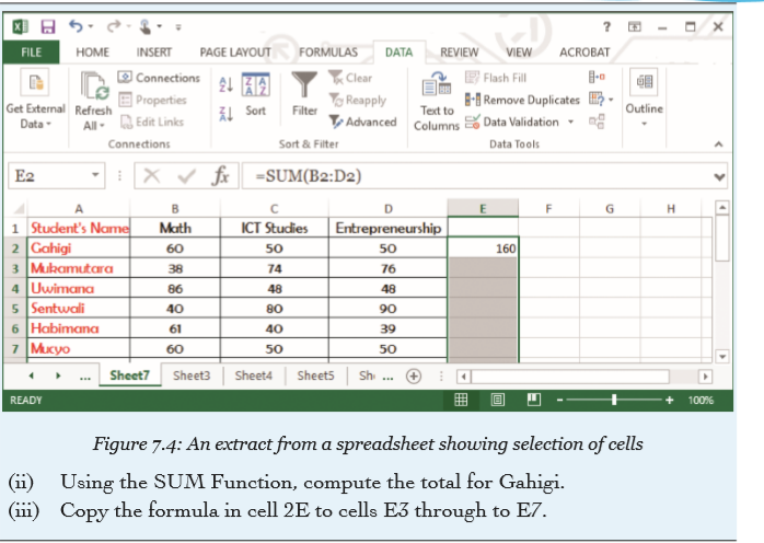
Figure 7.11: Students’ marks for CAT and examinations

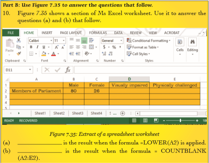
2. Figure 7.12 shows a list of items in a shop. Use it to answer the questions that follow.

Figure 7.12:  Costs of items 

(a) Open a new workbook and type the following data in a worksheet as it appears and save it as Costs on the desktop. 

(b) Use cell references to: 

(i) Compute the VAT for  cement using the cost in cell D6. 

(ii) Copy the formula entered in cell E2 to cells E3 to E5. 

(iii) Compute the total cost of cement, including VAT in cell F2. 

(iv) Copy the formula entered in cell F2 to cells F3 to F5. 

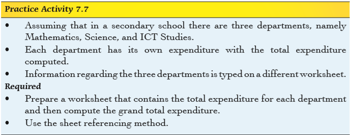
3.The  following is a hypothetical budget for three ministries in Rwanda. Use it to answer the questions that follow. 

(a) Open Microsoft Excel and type the data in figures 7.13, 7.14, and 7.15 in separate worksheets that are named Sheet1, Sheet2, and Sheet3 respectively. Save the Excel document as Budgets on the desktop.

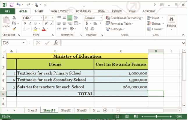
Figure 7.13:  Cost of items at the Ministry of Education

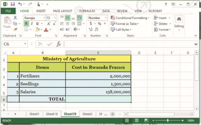
Figure 7.14:  Cost of items at the Ministry of Agriculture

Figure 7.15:  Costs of items at the Ministry of Health

(b) Calculate the total in each ministry. 

(c) Create another worksheet and key in the information shown in 

Figure 7.16:  Total cost of items for the ministries 

(d) Sheet reference the total for each ministry to appear on Sheet4. 

(e) Calculate the totals for all the ministries. 

(f) Change the cost of seedlings from 1,300,000 to 1,350,000 on Sheet1. 

(g) Observe the change in the worksheet you created for TOTALS. 

Save the changes in the document as Final. 

7.5 Functions 

Functions are inbuilt formulae that you can quickly use to perform calculations automatically.

As discussed in Unit 4, every function must have the following components: 

(i) Begin with an equal sign (=) or the at (@) sign. 

(ii) The name of the function. 

(iii) Cell addresses or data range. The data range is enclosed in parenthesis () or round brackets ().  It contains the cell addresses which have the information to be manipulated mathematically. The addresses can be separated by use of a colon or comma. 

The user can either type functions on their own or use the paste (fx) function. To activate this function, simply click on the fx label on the formula bar or click the Formulas menu on the menu bar and select Insert function from the Function Library group. A dialog box appears as shown in Figure 7.17(a).

Figure 7.17 : The Insert Function dialog box 

To make use of this function, do the following:

(i) Click on the cell where the result is to be displayed. 

(ii) Activate the Paste function to display the Insert Function dialog box shown in Figure 7.17. 

(iii) Select the function required to manipulate the data under Select a function: section. 

(iv) Click OK to apply and to open the Function Arguments dialog box. See Figure 7.18. 

(v) Excel automatically inserts the data range under Number1 box and displays all or some of the values to be manipulated besides the box.  However, the user has an option of either accepting the argument or typing their own. To type a new argument,click  on the box and delete the given range then type another one.

Figure 7.18: Function Arguments dialog box

 Excel has many functions which are divided into different categories. The following are some categories of functions: Mathematical, Logical and Text.

 Figure 7.19: Categories of functions

7.6 Mathematical Functions 
They are used to perform common mathematical operations. They include: SUM, AVERAGE, ODD, INT, ROUND, EXP, SQRT, POWER, MOD, MAX, and PRODUCT.
• SUM: This function adds all the values in a specified range of cells. The general syntax is =SUM(Number1, Number2…Number N).


• AVERAGE: It is used to calculate the mean of values specified in a selected range of cells. Empty cells within the range are ignored while those that have zero values are included. The syntax is: =Average(data range).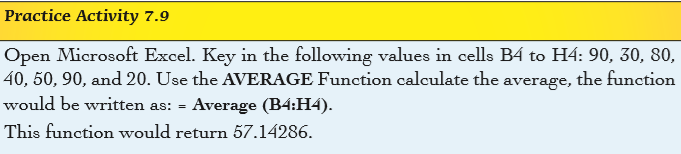

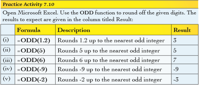
• ODD: It returns a value rounded up to the nearest odd integer. The general syntax is =ODD(number) where number is the value to be rounded. 

Note: 

(i) If number is non-numeric, ODD returns the #VALUE! error. 

(ii) Regardless of the size of the number, a value is rounded up when adjusted away from zero.

(iii) If number is an odd integer, no rounding occurs.

• INT: Rounds a number down to the nearest integer. The general syntax is  =INT(number) where number is the real number to be rounded down to an integer. 

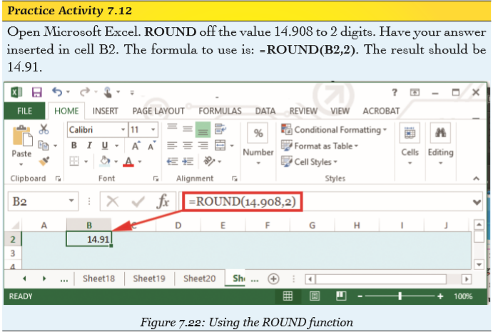
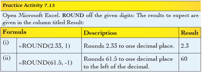
• ROUND: This function rounds off a number to a specified number of digits. The general syntax is =ROUND(number, num_digits) where number is the value to be rounded and num_digits is the number of digits in the fractional part of the number to which the result is to be displayed.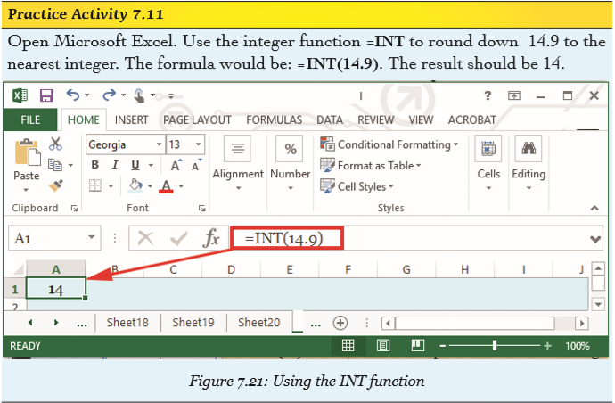 

Note: 

(i) If num_digits is greater than 0, then number is rounded to the specified number of decimal places. 

(ii) If num_digits is 0, the number is rounded to the nearest integer.

(iii) If num_digits is less than 0, the number is rounded to the left of the decimal point. 

• EXP: Returns “e” raised to the power of number. The constant e equals 2.71828182845904, the base of the natural logarithm. The syntax is =EXP(number) where the number is the exponent application to the base of “e”. 

• SQRT: This function returns a positive square root of a number. The general syntax is =SQRT(number) where number is the value for which the square root is to be obtained. If number is negative, this function returns #NUM! error.

• POWER: Return the result of a number raised to a power. The general syntax is =Power(number, power) where number is the base number which can be any real number while power is the exponent to which the base number is raised.
The “^” operator can be used instead of Power to indicate to what power the base is to be raised. 


• MOD: It returns the remainder after a number is divided by a divisor. The result obtained has the same sign as the divisor. The general syntax is: =MOD (number, divisor). Where number is the number for which the remainder is to be found and divisor is the number used for dividing.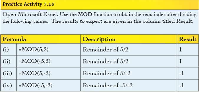 


• Note: If divisor is 0, MOD function returns the #DIV/0! error value.
• The MOD function can be expressed in terms of the INT function: MOD (n, d) = n – d*INT (n/d).
• MAX: The term Max refers to the function used for obtaining the maximum or largest value in a selected range of cells. If the selected range of cells contains no value, it returns a zero. The syntax is: =Max(data range).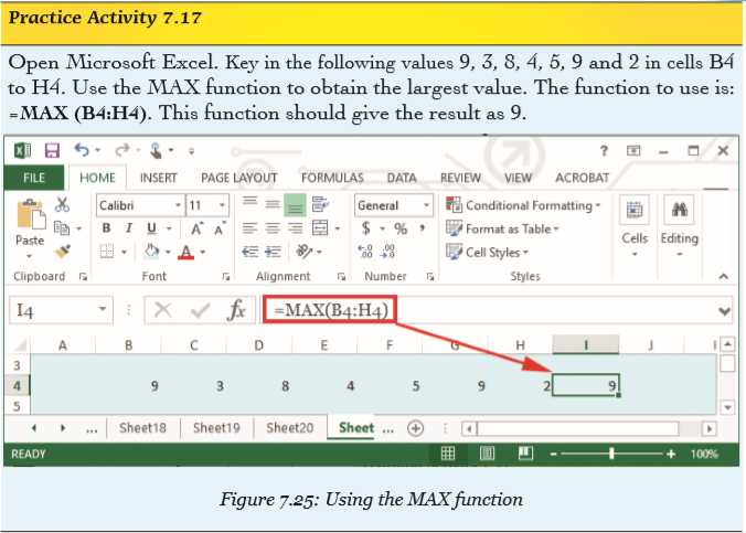


• PRODUCT: This function multiplies all the values within a specified range of cells. The general syntax is =Product(Number1, Number2… NumberN).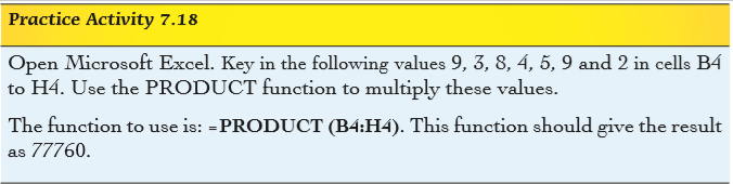


7.7 Logical Functions

 All logical functions return either the logical TRUE or logical FALSE when their functions are evaluated. They include AND, NOT, OR and IF.
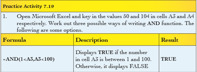
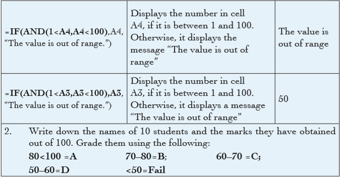
IF: This function evaluates a condition and returns one of the values in case it is found to be true and another value if it is false. When writing a formula using this function, there should be no space however long it is. The syntax for this function is dependent on the number of options and is as follows:

• For two options only:

® General syntax =IF(Condition, True, False)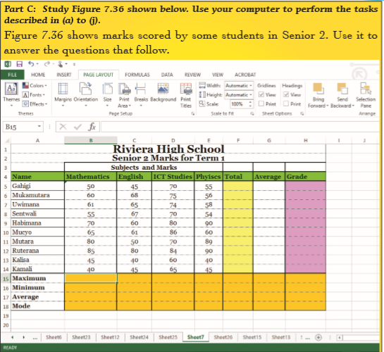

• For three options only: General syntax =IF(Condition1,Option1,IF(Condi tion2,Option2,Option3))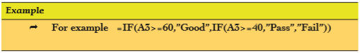

• For four options only:  General syntax =IF(Condition1,Option1,IF(Condit ion2,Option2,IF(condition3,Option3,Option4)))

Note: 

• It is important to note that the number conditions is always one less than the options. For example, if the options are four then the conditions are three because the last option is always the default. 

• Any open bracket should be closed at the end of the entire “IF” function. 

• No space should be used in the entire formula instead use commas. 

• AND: It returns TRUE if all values are TRUE and it returns FALSE if one or more values are FALSE. The syntax is =AND (logical1, logical2,...) where logical1 is the first condition to be evaluated and logical2 is the optional condition.

Notes: 

• Text or empty cells found within the selected range of cells are ignored. 

• If the selected range of cells does not contain any logical values, the function returns a #VALUE error. 

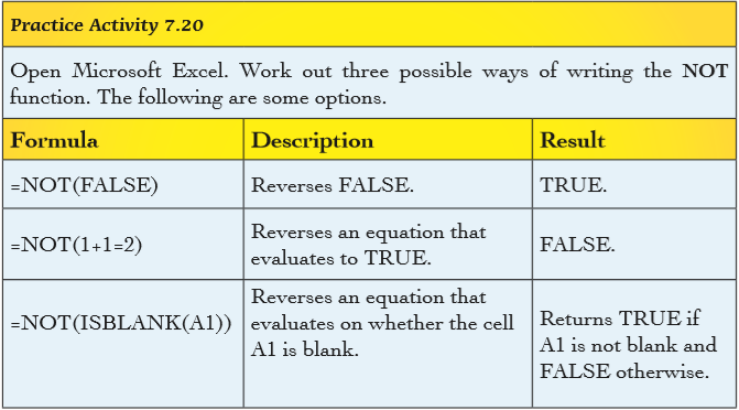
• NOT: Reverses the value of its argument, that is, it changes FALSE to TRUE and TRUE to FALSE. It is used to make sure a value is not equal to one particular value. The syntax of the function is =NOT(logical) where logical is a value or expression that can be evaluated to TRUE or FALSE.  If logical is FALSE, NOT returns TRUE and if logical is TRUE, NOT returns FALSE.

• OR:Checks whether any of the arguments are TRUE, and returns TRUE if any argument is TRUE and returns FALSE if all the arguments are FALSE. The syntax is:  

=OR(logical1, logical2, ...) where Logical1 is required and subsequent logical values are optional. Notes: 

• Text or empty cells given as arguments are ignored. 

• It returns a #VALUE error if no logical values are found. 

• Each logical condition must evaluate to TRUE or FALSE.

Solution

Solution with formulas 

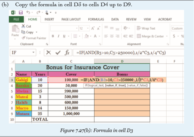
Solution showing calculated values

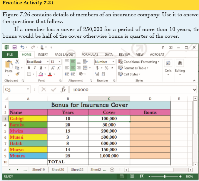
Figure 7.29: The bonus for each person 

7.8 Text Functions 

These are functions used in manipulating text strings. Examples of the text functions include: COUNTA, COUNTABLANK, UPPER, LOWER and REPLACE and SEARCH. 

• COUNTA: This function counts the number of cells that are not empty in a specified range (range: Two or more cells on a sheet. The cells in a range can be adjacent or nonadjacent.). It counts cells containing any type of information such as error values, text and empty text (“”).

For example, if the specified range contains a formula that returns an empty string, the COUNTA function counts that value. However, it does not count empty cells.

The syntax of the COUNTA function is: =COUNTA(value1, value2,…). Note: To count cells containing only values use COUNT function and to count cells that meet a given criteria, use COUNTIF function.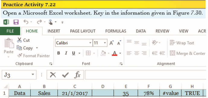 



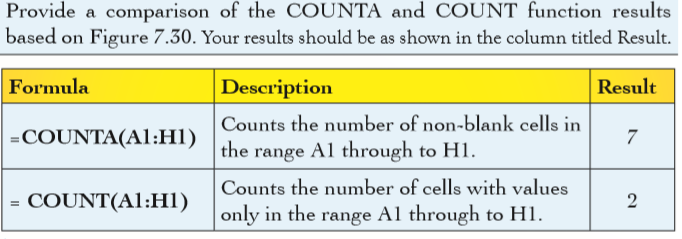
Figure 7.31: Comparison of COUNTA and COUNT functions

• COUNTBLANK: This function counts the number of empty cells in a specified range of cells as well as cells with formulas that return empty text (“”). However, it does not count cells with zero (0). The syntax is: =COUNTBLANK(data range).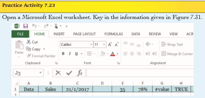 


Figure 7.32: Worksheet data containing different types of data

To count the empty cells only in the range, the formula would be written as =COUNTBLANK(A1:H1). The result is 1.

• UPPER: This function converts text to uppercase. The syntax of the function is: =UPPER(text) where text is the information to be converted to upper case which can be a reference or text string.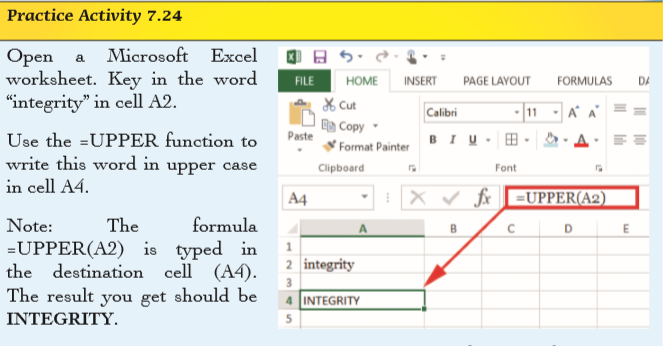

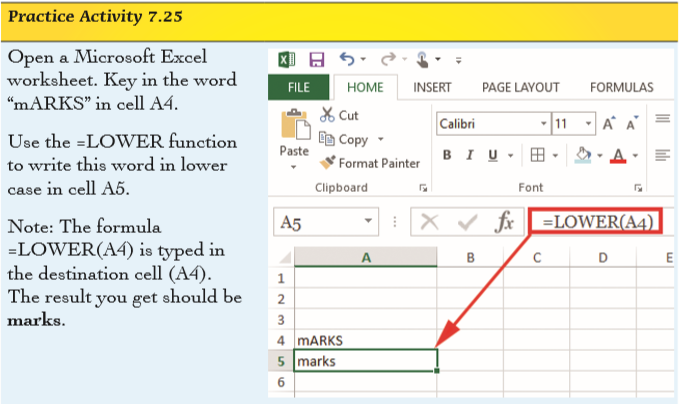
• LOWER: This function converts all uppercase letters in a text string to lowercase. The syntax of the function is: =LOWER(text) where text is the information to be converted to lower case. 

• REPLACE: It is used to substitute part of a text string based on the number of characters specified, with a different text string. The syntax of the function is:

=REPLACE(Old_text, start_num, num_chars, new_text) where:

 ® Old_text: This refers to the text containing some characters to be replaced. 

® Start_num: This is the position of the character to be replaced in the old_text. 

® Num_chars: is the number of characters in old_ text that the REPLACE function is to replace with new_text. ® New_text: is the text that will replace characters in old_text.

Figure 7.34: Using the REPLACE function

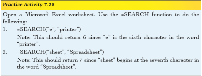
• SEARCH: This function locates one text string within a second text string then returns the number of the starting position of the first text string from the first character of the second text string. The syntax is: =SEARCH(find_ text,within_text_start_num) where: 

® Find_text is the text to be found.

 ® Within_text is the second text string where the text in the find_text is to be found.

 ® Start_num It is optional. It is the character number in the within_ text argument at which the search should begin. 

7.9 Conditional Formatting  

Conditional formatting enables the user to answer specific questions about the data in a worksheet. It can be applied to a cell range or an entire worksheet. It changes the appearance of a range of cells based on the conditions (or criteria).  

If the condition is true, the range of cells is formatted based on that condition. 

However, if the condition is false, the range of cells is not formatted. 

When a conditional format is created, it is possible to reference only other cells on the same worksheet or, in certain cases, cells on worksheets in the same workbook currently open.   

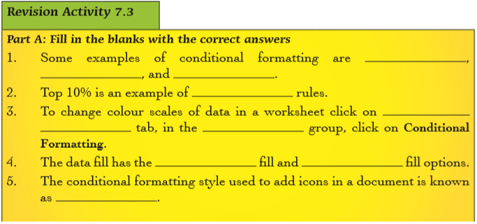
Conditional formatting, however, cannot be used on external references to another workbook. The following are some of the features of conditional formatting that can be applied: highlight cell rules, top bottom rules, data bars, colour scales, and icon sets. 

7.9.1 Highlight Cell Rules 

To apply Highlight cell rules, do the following: 

(i) Select the data where the highlight cell rules are to be applied. 

(ii) Click on the Home tab, in the Styles group, click on Conditional Formatting icon then point to Highlight cell rules. A drop down menu appears as shown in Figure7.37. The keyboard shortcut is as follows: LONG press ALT then H followed by L, and finally H key.

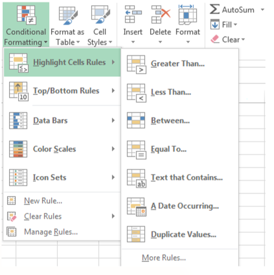
Figure 7.37: Highlighting cell rules 

(iii) Select the desired highlight cell rules option such as greater than or less than options. 

The following are the options available and their descriptions. 

Figure 7.38: Highlight cell rules 

(iv) Choose the desired format style from the with box as shown in Figure 7.39.

Figure 7.39: Different fill options that are available 

(v) Click OK to apply. 

7.9.2 Top/Bottom Rules

To apply Top/Bottom, rules do the following:

 (i) Select the data where the Top/Bottom Rules is to be applied.

 (ii) Click on the Home tab, in the Styles group, click on Conditional Formatting icon then point to Top/Bottom Rules. A drop down menu appears as shown in Figure 7.40. The keyboard shortcut is as follows: Long press ALT then H followed by L and finally T key.

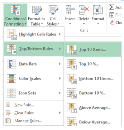
Figure 7.40: Applying Top/Bottom rules 

(iii) Select the desired top/bottom option such as Above Average options. 

(iv) Choose the desired format style from with box.

 (v) Click OK to apply. 

7.9.3 Data Bars 

To apply Data Bars do the following: 

(i) Select the data where the data bar is to be applied. 

(ii) Click on the Home tab, in the Styles group, click on Conditional Formatting icon then point to Data Bars.  A drop down menu appears as shown in Figure 7.41. The keyboard shortcut is as follows: Long press ALT then H followed by L and finally D key.

(iii) Select the desired data bars option. The format is automatically implemented. 

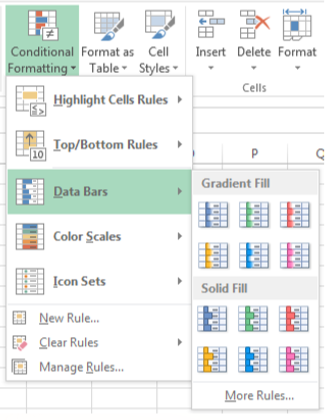
Figure 7.41: Applying data bars

7.9.4 Colour Scales 

To apply colour scales, do the following:

(i) Select the data where the colour scales is to be applied. 

(ii) Click on the Home tab, in the Styles group, click on Conditional Formatting icon then point to Colour Scales. A drop down menu appears as shown in Figure 7.42. The keyboard shortcut is as follows: Long press ALT then H followed by L and finally S key.

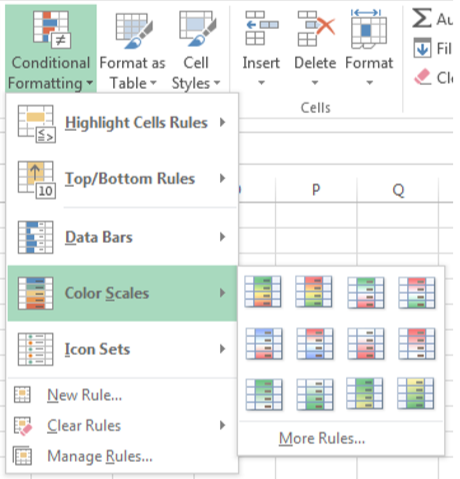
Figure 7.42: Applying colour scales

. (iii) Select the desired colour scales option.The format is automatically implemented. 7.9.5 Icon Sets To apply icon sets, do the following: 

(i) Select the data where the icon sets is to be applied. 

(ii) Click on the Home tab, in the Styles group, click on Conditional Formatting icon then point to Icon Sets. A drop down menu appears as shown in Figure 7.43. The keyboard shortcut is as follows: Long press ALT then H followed by L and finally I key.

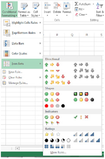
Figure 7.43: Applying icon sets 

(iii) Select the desired icon sets option. The format is automatically implemented on the cells containing values.

7.10 Definition of Key Words in this Unit

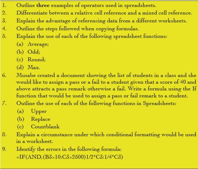
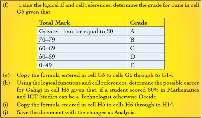
Revision Exercise 7