ICT

Key Unit Competency: By the end of this unit, you should be able to: 

Fill in a new empty map with data, use simple symbols, label features and attributes table, and navigate a map. 

Introduction 

Maps are important ways of organising and displaying data. 

6.1 Creation of Maps

Maps contain many kinds of data such as world imagery, street maps, topographic data, and base maps. The data on a map is organised into layers, which are drawn on the map in a particular order. Each map is displayed in a Page Layout view or window where graphic elements such as legends, North arrows, scale bars, text, and other graphics, are arranged.

Layers give a layout of geographical features added to a map. Layers refer to data that is stored in the Data folder. Layers also define how a set of geographical features will be drawn when they are added to a map. They also act as shortcuts to the storage location where the data is stored. 

Generally, making maps in ArcMap takes the following steps: 

(i) Load Geospatial data into ArcMap. 

(ii) Identify the features and attributes to present. 

(iii) Define how to show the data. 

(iv) Add map components. 

(v) Export the map. 

ArcMap allows one to work with geographic data in maps, regardless of the format or location of the underlying data. With ArcMap, one can assemble a map quickly from predefined layers. Data can also be added from coverages, shapefiles, geodatabases, grids, images, and tables of coordinates or addresses. 

ArcCatalog is another GIS application that is designed to work with ArcMap. It is used to browse, organize, and document geographic data. It is also used to easily drag and drop it onto an existing map in ArcMap.

6.1.1 Introducing ArcCatalog 

To start the ArcCatalog application, proceed as follows: 

(i) Click the Start button on the taskbar. 

(ii) Point to Programs to display the Programs menu. 

(iii) Point to ArcGIS. 

(iv) Click ArcCatalog.

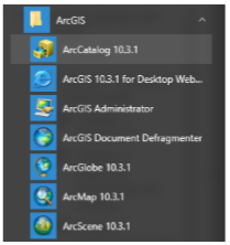
Figure 6.1: Launching ArcCatalog 

The ArcCatalog window starts and the two panels in the ArcCatalog window are displayed as shown in Figure 6.2 below.

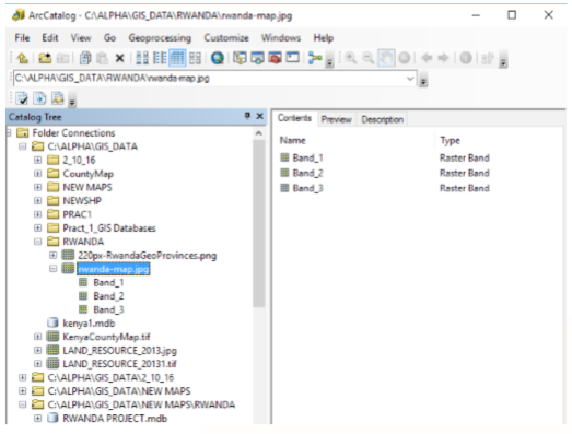
Figure 6.2: The ArcCatalog Window 

The Catalog tree on the left side of the ArcCatalog window is for browsing and organising the GIS data. The contents of the current branch (Rwanda-map.jpg) are displayed on the right side of the Catalog window.

When more information about a branch of the Catalog tree is needed, one can use the Contents, Preview, and Description tabs to view the data in many different ways.

For example, clicking on the Preview tab for the selected branch displays the view shown in Figure 6.3 below.

Figure 6.3: Previewing the contents of a Branch 

By default, ArcCatalog recognises many different file types as GIS data including shapefiles, coverages, raster images, TINs, geodatabases, projection files, and so on. 

 If the list of the recognised file types does not include a file type that is being used in GIS analysis, ArcCatalog is customised to recognise additional file types, for example, text files as GIS data.

6.1.2 Maps and layers

 Maps and layers are the main ways of organising and displaying data in ArcGIS.

Maps, such as printed paper maps, can contain many kinds of data. Data on a map is organised into layers, which are drawn on the map in a particular order

Each map contains a Page Layout where graphic elements, such as legends, North arrows, scale bars, text, and other graphics, are arranged. The layout shows the map page as it will appear in print.

Layers outline how a set of geographic features are drawn when they are added to a map.

If geographic data is stored in a central database, then maps and layers can be created that refer to the database. This makes it easy to share maps and layers with other related users, eliminating the need to make duplicate copies of your data for each user.

ArcGIS has tutorial data which we need to know where it has been installed on the system. 

6.1.3 Adding Data to a Map

Make a connection to the tutorial data Now we will add a connection to the folder that contains the tutorial data. This new branch in the Catalog tree will remain until it is deleted. 

(i) Click the Connect to Folder button.

Figure 6.4: Connecting to a Folder from ArcCatalog 

After clicking the button, a window opens. It allows one to navigate to a folder in the computer or to a folder in another computer in the network. 

(ii) Navigate to the ArcGIS\ArcTutor\Getting_Started\Greenvalley folder on the drive where the tutorial data is installed. Click OK.

Figure 6.5: Connecting to the Tutorial Data 

The new connection is displayed as a branch in ArcCatalog tree as shown in Figure 6.6 below.

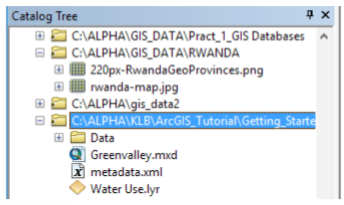
Figure 6.6: The new Connection in the Catalog Tree The Greenvalley folder has a special icon to show that it contains GIS data. 

6.1.4 Open the Greenvalley map 

Double-click Greenvalley in the Catalog tree. Double-clicking a map in the Catalog tree opens the map in ArcMap. 

One may also want to start ArcMap without opening an existing map. This is done by clicking the ArcMap Launch button  in ArcCatalog.ArcMap can also be launched from the start menu just like ArcCatalog.

6.1.5 ArcMap 

ArcCatalog is used for browsing, organising, distributing, and documenting GIS data. ArcMap is the tool for creating, viewing, querying, editing, composing, and publishing maps. Maps can present several types of information about an area at once. This map of Greenvalley contains three layers that show public buildings, streets, and parks. The layers in this map are listed in the table of contents. Each layer has a check box that lets you turn it on or off.

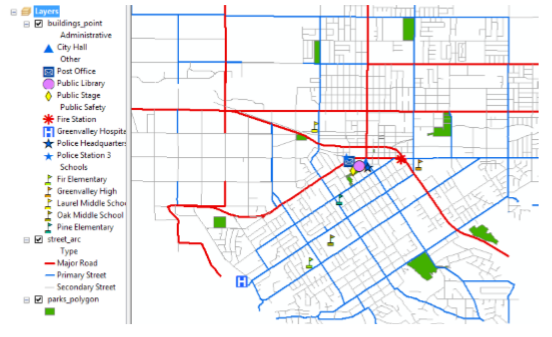
Figure 6.7: Layers Displayed in ArcMap 

Within a layer, symbols are used to draw the features. In this case, buildings are represented by points, streets by lines, and parks by areas. Each layer contains two kinds of information. 

(i) Spatial information: This kind of information describes the location and shape of the geographic features. 

(ii)  Attribute information: This kind of information tells you about other characteristics of the features. 

In the park layer, all the features are drawn with a single green fill symbol. This single symbol lets one identify areas that are parks, but it does not tell anything about the differences between the parks. 

In the street layer, the features are drawn with different line symbols according to the type of street that the lines represent. This symbol scheme lets you differentiate  

streets from other types of features and tells you something about the differences between the features as well.

6.1.6 Adding a layer to a map 

We will start by adding the Water Use layer to the in ArcMap map.

 (i) Position the ArcMap and ArcCatalog windows so that both windows can be seen. 

(ii) Click the Water Use layer in ArcCatalog and drag it onto the map in ArcMap. One can click and drag any layer from the ArcCatalog tree onto an open map in ArcMap. 

The map now shows a new water use layer as shown in Figure 6.8 below.

Figure 6.8: Addition of a new water use layer 

One can add raw geographic data to a map just as easily as you can add a layer.

6.2 Display of a Layer 

6.2.1 Adding Features and Symbolising Layers 

Symbology is a set of conventions, rules, or encoding systems that define how geographic information is represented with signs and different colours on a map.

A characteristic of a map feature may influence the size, colour, and shape of the symbol used. Figure 6.9 below shows examples of custom symbols common in maps.

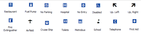
Figure 6.9: Example of Symbols used in Maps. 

Symbols can be applied into layers in different ways depending on the type of data.

The following are some of the forms used: 

(i)  Single symbol: All features are represented in the map with a common symbol.

(ii)  Unique values: A different symbol is applied to each category of feature within the layer.

(iii)  Graduated colours: Variety of colours are used to show differences in feature values. 

(iv) Dot Density Symbols: Thematic dot density maps use dots or points to show a comparative density of features over a map based on values stored in the fields. Attribute values determine the number of dots displayed in the polygon feature.  

(iv)  Graduated symbols: These are common symbols that are used to represent qualitative information of different values using symbol with varying sizes. Using graduated symbols, the quantitative values for a field are grouped into ordered classes. Within a class, all features are represented with the same symbol.

 6.2.2 Adding Features

When features are added directly from a coverage, shape file, or database, they are all drawn with a single symbol. Let us go back to the Green valley example. The data will be added from a database in this case. 

(i) Position the ArcMap and ArcCatalog windows so that both can be seen. 

(ii) Click the plus sign (+) next to the Data folder in the Catalog tree to view the contents of the folder. 

(iii) Click the plus sign (+) next to GreenvalleyDB. 

(iv) GreenvalleyDB is a geodatabase that contains the remainder of the data to be used. This data is organised in five feature datasets, namely Hydrology, Parks, Public Buildings, Public Utility, and Transportation.

(v) Click the plus sign (+) next to Public Utility.
(vi) Click Watermains_arc and drag it onto ArcMap.

Figure 6.10 below represents the ArcCatalog window showing the steps followed to access the data in the geodatabase.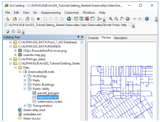 

Figure 6.10: ArcCatalog Window showing the location of the Greenvalley Database 

Watermains_arc layer is then dragged and added to the ArcMap window. It appears as shown in Figure 6.11 below.

Notice that, the map now has four layers: Building_point, Watermains_arc, street_arc, and parks_polygon.
The Watermains_arc layer features are represented using a single symbol which is a uniform line. In this case, the features are polyline shapes that represent the pipes in the water distribution system.

The features in the Building_point layer are represented using unique values, where a different symbol is applied to each category of feature within the layer. The represented features include city hall, post  office, public library and schools among others.

Following the steps above, add the water use layer from the catalog tree.

Figure 6.12 below represents the added layer.

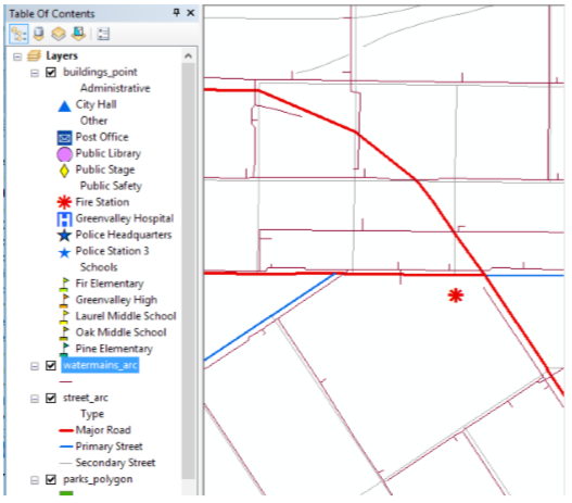
Figure 6.11: ArcMap window showing the added Watermains_arc layer

Figure 6.12: The water use layer added represented using Graduated colour scheme.

The features in the water use layer are represented using the graduated colour scheme. Zero (0) represents nil water use, 1-2 represents light water use and 7-8-9 represents heavy water use. For example,the school and the fire station are heavy water consumers and they are represented using colour code 7-8-9 as indicated in the table of contents.

The street_arc layer also represents the different classes of roads using different colours. Figure 6.13 below shows the colour graduated scheme differentiating the countries neighboring Rwanda.

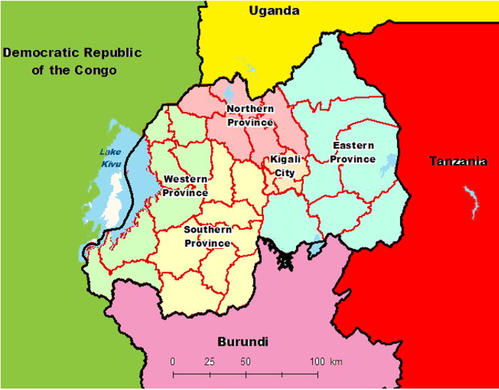
Figure 6.13: Graduated Color Scheme Differentiating Rwanda’s Neighboring Countries 

6.2.3 Editing the feature Symbols 

Sometimes, the size, colour and shape of the features need to be changed to give the correct representation. To achieve this, proceed as follows:

(i) Right-click the layer title (for example Watermains_arc) in the ArcMap table of contents and click Properties. The layer Properties dialog box shown in Figure 6.14 below appears. It can be used to inspect and change a wide variety of layer properties. 

(ii) Click the symbology tab. The symbol scheme for the layer, as well as its appearance in the table of contents can be edited from this tab.

 

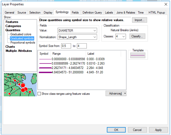
Figure 6.14: Layer Properties Dialog box 

(iii) Click Quantities. The panel changes to give controls for drawing with graduated colors, graduated symbols, and proportional symbols. 

(iv) Select Graduated symbols option and click the Value dropdown arrow and click DIAMETER. By default, ArcMap assigns the data to five classes using the Natural Breaks classification (Jenks’ method).

The classes can be adjusted to the desired number. Now the width of the line symbols indicates the diameter of the water mains.

If one wants to change the water mains colour (for example to be ginger pink), click on the template button and select the desired colour.

 After clicking, apply and then okay, applies the changes to the selected layer in the map as shown in Figure 6.15.

Figure 6.15: Water main Pipes represented using graduated symbols to show different sizes. 

From the geodatabase, add another layer for Water mains_nodes. This layer will represent the water points. From the layer properties dialog box, edit the colour, shape and size of the nodes and apply the changes. Figure 6.16 below represents the changes.

Figure 6.16: Water nodes represented using the Dot Density Symbols.

6.2.4 Add/Remove Labels of a Layer

Progressively, layers have been added to the Greenvalley map as shown in Figure 6.16 above. The table of contents usually displays the active layers in a map. In a Map, to remove the label of a layer, uncheck the dialogue box, next to the layer label. Figure 6.17 below shows the label for water use layer unchecked. The map will not display the water use scheme of the town.

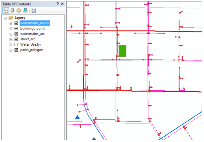
Figure 6.17: Removal of Layers from a Map with layer of Water Use unchecked. 

To add the layer for the cities, just check the Checkbox against the layer and the feature appears in the map.

6.2.5 Layer Properties

 Layer properties usually define the display and feature of a layer. All the aspects of the layers can be controlled through Layers properties. The properties of a layer can be updated and accessed through the layer Properties dialog box. The properties set are different for different types of geographic data. For example, when designing 3D maps, additional properties, such as elevation of the layer from the surface are set. 

To change these settings, select a layer in the Table of Contents pane, right-click on it and select properties. The Layer properties dialog box in Figure 6.18 appears.

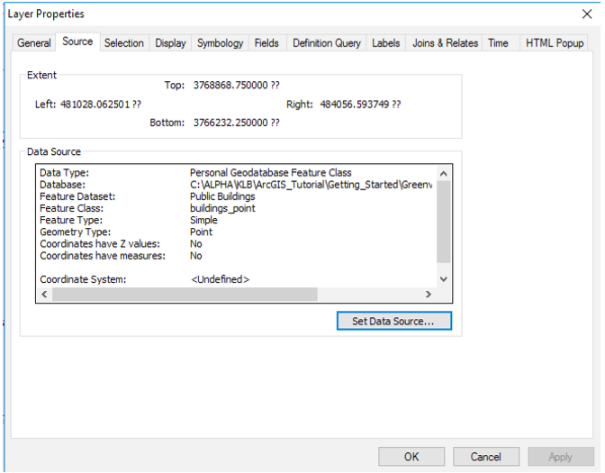
Figure 6.18: The Source tab in the Layer Properties dialog box. 

The tabs on this dialog box are specific to the type of layer. The following are some of the properties for feature layers one can set using the Layer Properties dialog box. The tabs in the Layer Properties dialog box for Feature layers can be described briefly as follows: 

(i) General: This tab allows the recording of layer properties such as layer name,its description, and set credits. It also specifies scale-dependent drawing properties. 

(ii) Source: This tab allows viewing of the extent of the data. The source of the data can be viewed and changed from this tab. 

(iii)  Selection: This tab allows the setting of how features in a specific layer are highlighted when they are selected. The symbol shape and color can be changed in this tab. 

(iv) Display: The tab is used for setting the symbol transparency, display field expressions, support hyperlinks using fields, and exclusion of features from the drawing.

(v) Symbology: This tab provides options for assigning map symbols and rendering the data. The tab provides options for drawing all features with one symbol, using proportional symbols, using categories based on attribute values, the use of quantities, colour ramps, or charts based on attributes and the use of representation rules and symbols.

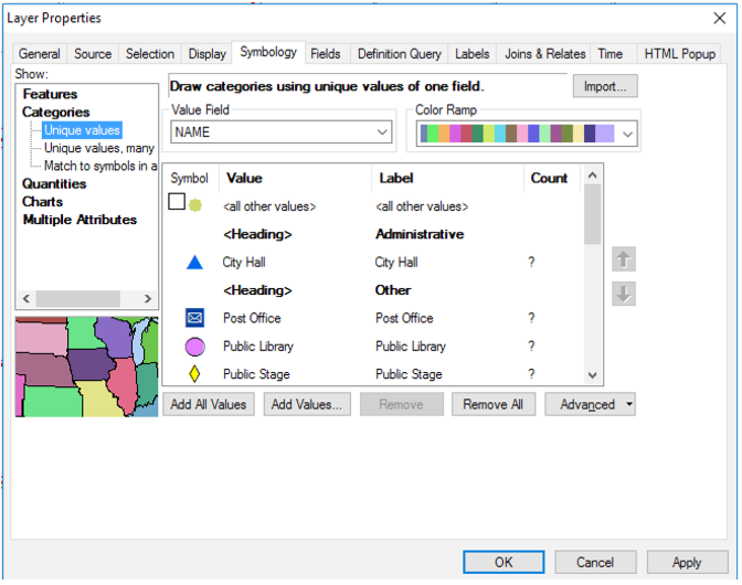
Figure 6.19: Symbology. 

(vi) Fields: The tab is used to set characteristics about attribute fields. Other options include creation of aliases.  An important aspect is to set alias names for visible fields that make it easier for users to work with feature attributes. One can also format numbers, and make fields invisible.

(vii) Definition Query: This tab allows one to specify that a subset of a feature is used inthe layer. With the Query Builder dialog box, one can create an expression to select particular features of a dataset to be used in a layer. 

(viii) Labels: This tab allows one to turn on a layer’s labels, build label expressions, manage label classes, and set up the labelling options for label placement and symbology. Alternatively, one can set labelling properties for all layers within the map using the Label Manager. 

(ix) Joins and Relates: This tab allows one to join or relate attribute tables to the layer’s feature attribute table.

(x) Time: This tab is used to specify the time properties of time-aware layers.
  
(xi) HTML Popup: This tab is used to specify how pop-up lists are generated when you click a feature to display information about it.

When working with one symbol at a time, any of its properties can be changed and even restructured by adding or removing components.
When more than one symbol is selected, one can only change basic symbol properties, which vary based on symbol type as shown in the table below: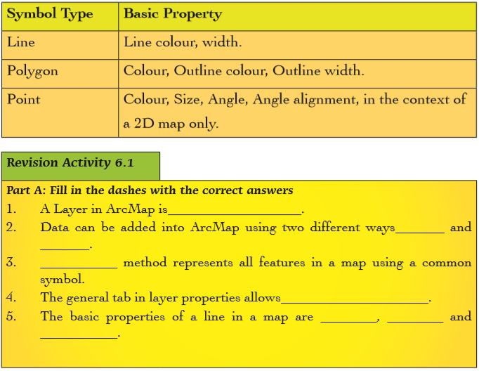  

6.3 Attribute Table

6.3.1 Adding a Field to a Table 

Follow the following procedure to add a field to a table. 

(i) Click the Add Data button  and browse to the data to be added. 

(ii) Open the attribute table of this file by right clicking on the layer and choosing the Open Attribute Table from the drop down menu as shown in Figure 6.20.  Note that when you let the cursor hover on the Open Attribute Table from the drop down menu, a help tip showing the keyboard shortcut appears as shown in Figure 6.21.

Figure 6.20: The window for opening the Attribute Table

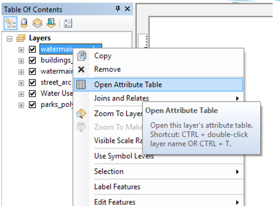
Figure 6.21: The window for opening attribute table showing the help tip.

(iii) Once you click on Open Attribute Table, the window shown in Figure 6.22 appears. In the attribute table, click on the Table Options in the top left corner and choose Add Field.

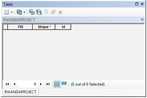
Figure 6.22: The Attribute Table

(iv) To create a new field called AREA1, click on the Table Options in the top left corner and choose Add Field. Type in the name of the field (AREA1) and click OK. Figure 6.23 shows how a field is added.

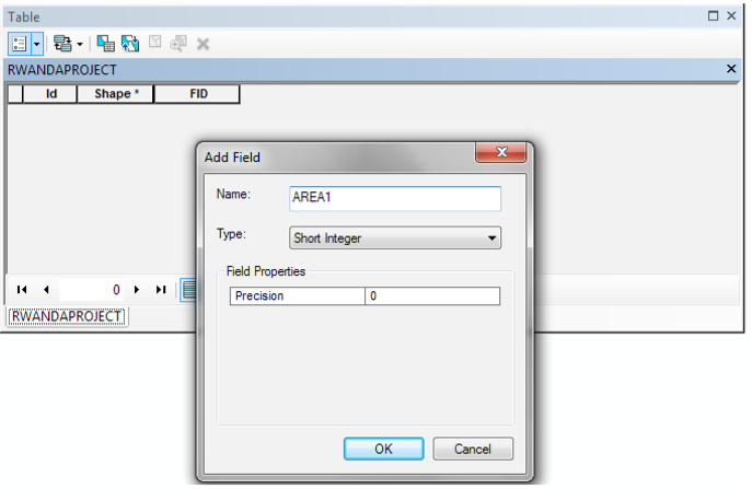
Figure 6.23: Adding a Field to a Table 

Field is a column in an attribute table that contains information for each feature. 

Each row in a basic table contains the following: 

• FID – Feature ID 

• Shape–Point, Polyline, Polygon

• ID – initially 0 but can be reset by user 

Field types can be:

• Integers (short or long) 

• Decimal numbers (floats or doubles)

• Text

• Date 

• Binary Large Objects (BLOB)

• Global Unique Identifier (GUID)

(v) For the created field called Area, use a built-in function to populate this field. Right-click on the field name and choose Calculate Geometry

• For the option to work, populate the values of the field to be geometric values derived from the features that the table represents such as area, perimeter, and length among others. 

• The dialog box that appears lets one decide whether the records will be calculated or just the selected records. 

• Note that when you let the cursor hover on the Calculate Geometry from the drop down menu, a Help Tip giving further details appears as shown in Figure 6.24.

Figure 6.24: Selecting the calculate Geometry feature. 

• Probably a warning about calculating outside of an edit session will appear. Click Yes to ignore it and continue. 

• In the Calculate Geometry dialog box, the area will be calculated. 

6.3.2 Sorting Records in Attribute Table 

Sorting the rows in a table allows information about the contents to be derived more easily. 

For example, if the information is about the population of a country in a particular period, after sorting a column’s values in ascending order, the values are ordered from A to Z or from 1 to 10. 

With descending order,a  column’s values are arranged from Z to A or from 10 to 1. To sort records: 

(i) Click the heading of the field column whose values are to be used for sorting.

(ii) Right-click the selected field’s heading and click Sort Ascending or Sort Descending. The drop down menu in Figure 6.25 will appear. 

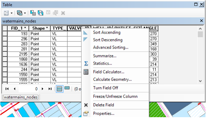
Figure 6.25: Sorting Records

 Note that when you let the cursor hover on the Sort Ascending from the drop down menu, a Help Tip giving further details appears as shown in Figure 6.26 below.

(iii) Sort the values in the field FID_1 in ascending order (A–Z) (1–9). The data before and after sorting appears as shown in the Figure 6.27 below.

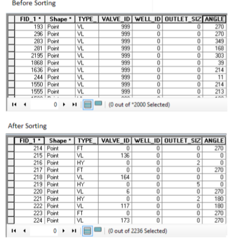
Figure 6.27: Results after Sorting Record 

6.3.3 Freezing and Unfreezing a Column 

Freezing a column helps in showing how attributes for the same feature are related with respect to one or more key fields (that are frozen). When a column gets frozen, it is always displayed even when scrolling horizontally in the table. To freeze a column, do the following:

 (i)  Click the heading of the column to freeze. 

(ii) Right-click the selected column’s heading and click Freeze/Unfreeze Column. The column is frozen. 

Figure 6.28 below shows the process of freezing the column named NAME.

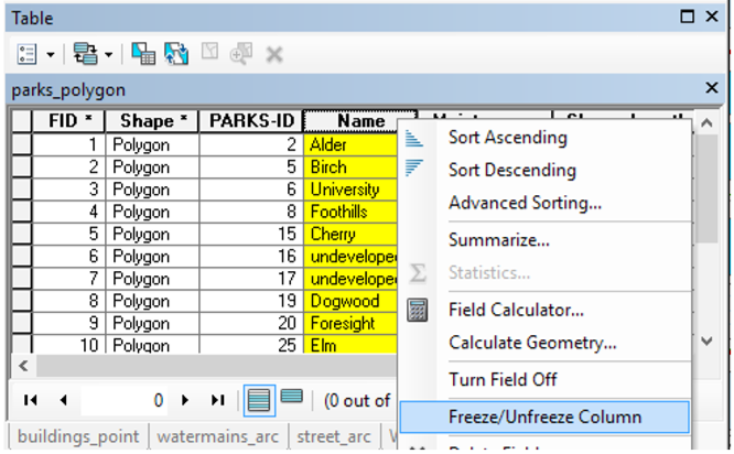
Figure 6.28: Freezing a Column 

Figure 6.29 shows the same column after it has been frozen.

Figure 6.29: Frozen Column

(iii)  Right-click the column heading of the frozen column and click Freeze/Unfreeze Column to unfreeze the column. 

6.4 Querying Data 

A request that examines features or tabular attributes based on user-selected criteria and displays only those features or records that satisfy the criteria is called data querying.

Information about features can be retrieved in different ways. Features can be identified by clicking on them to display their attributes.

The user can find features by using known information about the feature in order to search the map for that particular feature.

There are different ways of retrieving information about features in ArcMap. The user can identify features by clicking on them in order to display their attributes.

Alternatively, the user can select features by clicking on them to highlight and then look them up from their records in the layer attribute table. The user can find features by using known information about the feature in order to search the map for that particular feature.

6.4.1 Identify 

The identify tool offers a quick way of getting information about a single feature. To use the Identify tool, proceed as follows: 

(i) Select the Identify tool from the Tools Toolbar. 

(ii) Within the map, click on the feature of interest in order to view the attribute information for that particular feature.

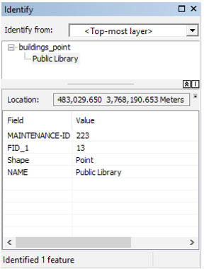
Figure 6.30: Using the Identify Tool

6.4.2 Measure 

This tool allows distances, areas, and feature locations on a map or scene to be measured. One can draw a line to measure length, a polygon to measure area, or click an individual feature to get measurement information. 

Once the user highlights what is to be measured, they click on the map. For example, to measure the distance of a line feature such as a river, the first click begins a line segment, and the next click ends that segment and begins another. Double-click to finish measuring. 

One can measure any number of segments in a sequence. That means to measure the distance of the river as it meanders, click each point where the river curves to make a segment. 

Downstream the next curve will require another click. A cumulative sum for the distance or area displays as part of the results. The results can be copied and pasted for use in other application. 

To measure in a map; 

(i) Click the Measure tool. 

(ii) Choose a measuring tool and click the map to begin measuring. 

• Distance: Click the map to measure the straight-line distance between two or more points. Figure 6.31 shows measuring of distance in a map.

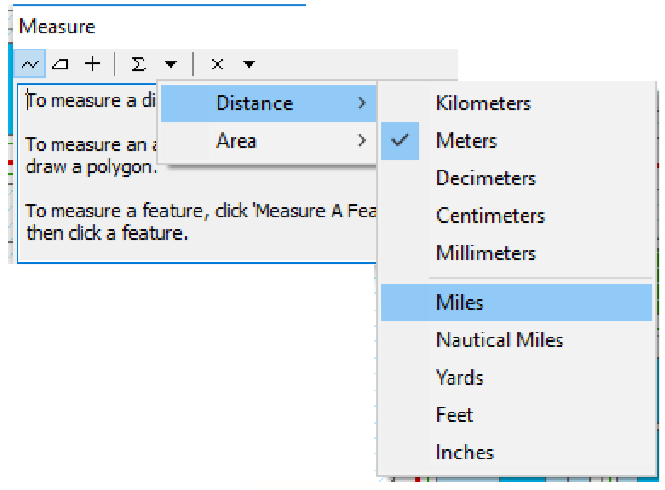
Figure 6.31: The Measure Dialogue Box.

Figure 6.32: Measuring Distance 

• Area: Select the tool for measuring area. Click the map to measure the area of a given locality, for example, a forested area. Identify the starting point on the map, and then successively keep clicking along the edges of the area to be measured until the starting point. The dimensions of the polygon shape will be displayed. Figure 6.33 shows measuring of an area in a map.

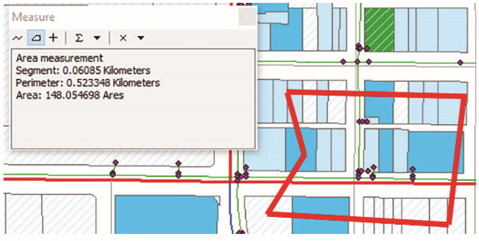
Figure 6.33: Measuring Area in a Map 

6.4.3 Go to XY This tool is used for typing in XY coordinates of a location and navigating to them. The coordinates entered can be: 

(i)  Longitude-Latitude: This is giving the Global Positioning System (GPS) of a given location. 

(ii)  Values in the map document’s coordinate system. These refer to the values of the given location. 

(iii)  Military Grid Reference System (MGRS) coordinates: The military grid reference system (MGRS) is the geocoordinate standard used by NATO militaries for locating points on the earth. 

(iv)  Universal Transverse Mercator (UTM) coordinate notation: This is a system that uses a two-dimensional Cartesian coordinate system to give locations on the surface of the Earth. The MGRS is derived from the Universal Transverse Mercator (UTM) grid system. On the tools toolbar, click the Go To XY button  to open the Go To XY dialog box, which is shown in Figure 6.34.

Figure 6.34: Go To XY dialogue Box. 

The dialogue box can be used to pan to, zoom to, flash or add call out to a location. Figure 6.35 below is showing a point with coordinates X (612,000) and Y (9,835,000) having a call out.

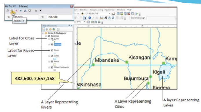
Figure 6.35: A location with XY coordinates

6.4.4 Hyperlink 

Hyperlinks allow access to documents or web pages related to features. These hyperlinks can be accessed for each feature using the Hyperlink tool on the Toolbar.  Hyperlinks have to be defined before using the Hyperlink tool. Hyperlinks are usually of three types:

(i)  Document: Clicking a feature with the Hyperlink tool opens a document or file using its appropriate application (such as Microsoft Excel). For example, on selecting a hyperlinked feature such as a school, a linked Microsoft Word document pops up to provide more information on the school. 

(ii)  Universal Resource Locator (URL): On clicking a feature with the Hyperlink tool, a web page is launched in the web browser. For example, when a hyperlinked feature like the Kigali Genocide Memorial Centre is selected with the hyperlink tool, a linked website pops up to give more details about the centre. 

(iii)  Script: On clicking a feature with the Hyperlink tool, a feature value is sent to a script.

 Hyperlink for a feature can be defined in a layer either by using field-based hyperlinks or by defining a dynamic hyperlink using the Identify tool. To define field-based hyperlink properties: 

(i) Right-click the layer for which the hyperlink properties are to be set and choose Properties. 

(ii) Select the Display tab on the Layer Properties dialog box. 

(iii) Check Support Hyperlinks using field. Figure 6.36 below show the dialogue 

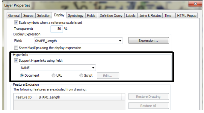
Figure 6.36: Setting Hyperlink Properties 

The hyperlink field has to be set up before specifying hyperlinks in this dialog box.  

For example, if a particular web page needs to be launched whenever a feature is clicked with the Hyperlink tool, first add a text field to the attribute table of this layer to contain the URLs associated with each feature. 

Then in the dialog box, check the Hyperlink option, choose the field from the drop-down list of fields, and choose the URL radio button option. 

The values of the field chosen to provide hyperlinks can include the full path to the target document or the full URL of the target web page.  

Alternatively, the value may just contain the name of the target document or web page, and one can use the Hyperlink Base property to specify the path or URL where the target can be found. Omit the “(http://)” part of the URL. 

If a protocol different from http is to be used, then it must be included in the protocol at the beginning of the URL. 

(iv) Select the field name you wish to use for the hyperlink and the link type, either document, URL, or Script. 

(v) If you choose to use Script, use the Edit button to write your script using JScript or VBScript. Click OK. 

(vi)  Click OK or Apply on the Layer Properties dialog box. 

Fig. 6.37: Hyper Link Script Dialogue Box

Note: 

(a)  The dialog box allows building of a script that will launch a hyperlink. The script should be coded using the rules of the scripting language selected in the Parser drop-down list. The script can include any valid statements supported by the selected scripting language.

(b)  Fields are enclosed in square brackets [ ], irrespective of the data type of the layer’s data source.

(c)  The hyperlink script is written as a function, which can contain programming logic and multiple lines of code. 

(d) The default functions utilise the ShellExecute function, which is part of the MSDN library.

• Microsoft ShellExecute Function Reference 

• Microsoft VBScript Language Reference 

• Microsoft JScript Language Reference 

• Python Language Reference

(e)  Click OK or Apply on the Layer Properties dialog box. You can define a hyperlink for the features in a layer either by using field based hyperlinks or defining a dynamic hyperlink using the Identify tool.

A hyperlink can be added to a feature using Identify tool. To define field-based hyperlink properties, do the following: 

(i) Right-click the layer for which you want to set hyperlink properties and choose Properties.
(ii)  Select the Display tab on the Layer Properties dialog box.
(iii)  Check Support Hyperlinks using field. Alternatively, you can also add a hyperlink as follows:

(i) Click the Identify tool on the Tools toolbar.
(ii) Click the feature for which you want to define a hyperlink.
(iii) Right-click the feature in the Identify window and click Add Hyperlink.
(iv) Specify the desired hyperlink target. Suppose we want to hyperlink the Public Library, we click on it with the Identify tool as shown in Figure 6.38. 
Figure 6.38: Adding Hyperlink using the Identify Tool

(v) On clicking Add the Hyperlink, the dialogue box shown in Figure 6.39 below appears. 

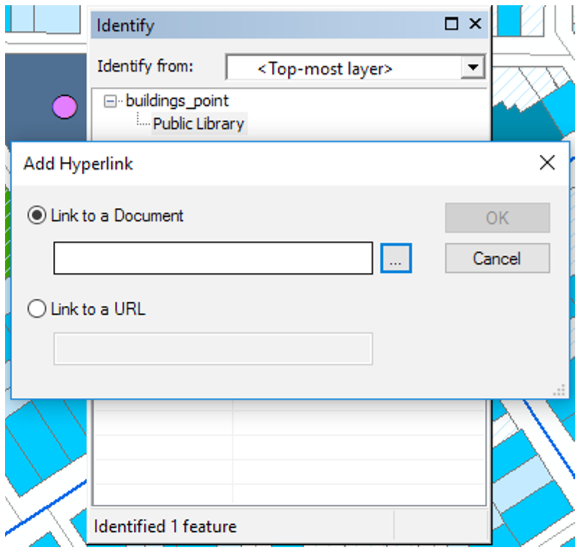
Figure 6.39: Hyperlinking a Document or URL 

(vi) Browse to link the document or type the URL and then click OK. 

(vii) To access the linked document, using the hyperlink tool, click on the feature; that is, Public library. The linked document opens. Moving the hyperlink tool over the feature displays the name of the linked document as shown in Figure 6.40.

Figure 6.40: Displayed name of the hyperlinked document.

6.4.5 Select Features 

The Select Feature tool allows the selection of features based on various categories relative to other features. Figure 6.41 below is showing the different options selections can be performed.

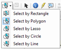
Figure 6.41: Different Select Options

For example:

 If the number of schools within a certain area is to be found, and the area is mapped by a boundary, all the schools within that area can be selected.

To find all the students who live within a 10-kilometre radius of the school and who made a recent improvement in their academic performance so as to give awards, proceed as follows: 

(i) First select the students within this radius (select by location).
(ii) Refine the selection by finding those students who have made a recent improvement according to the recently released results. 
The example of the selection given above is known as select by attribute. The attributes in the above example are students selected by:
• Living within a 10-kilometre radius of the school.
• Made improvement in their academic performance. 

6.4.6 Spatial Thinking 

Spatial thinking is about how we think about and understand our environment. A spatial thinker visualises and understands his or her environment from various angles. We apply spatial thinking when we create representations such as maps.

6.6 Definition of Key Words in this Unit

Revision Exercise 6