ICT

Key Unit Competency: By the end of this unit, you should be able to:

Manage a window, sort and filter data in a spreadsheet.

Introduction 

The Microsoft Excel worksheet is made up of many columns and rows. Information entered in a worksheet may occupy many columns and rows such that it cannot be viewed in one screen.

This topic introduces the learner to ways of dealing with large data and information in a worksheet such as sorting, filtering, freezing, and splitting worksheets. 

5.1 Freeze panes 

If  information in the worksheet stretches down or across more than one screen, normally as the user scrolls down or across the worksheet, the information keeps on disappearing to the top or to the left as the ones towards the bottom or right of the screen are displayed.

The freeze command is used to permanently display selected rows or columns. For example, the column or row titles can be frozen to ensure that the data displayed is viewed with the correct title after scrolling.

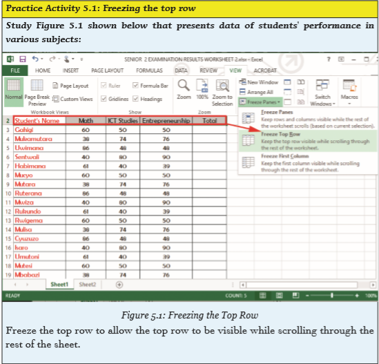
5.1.1 Freeze Top Row 

If a worksheet contains a large amount of information, the top row containing the titles or column headings could be frozen to keep it visible while scrolling through the rest of the worksheet. To freeze the top row, do the following: 

(i) Select a cell in the top row where the freeze command is to be applied. 

(ii) Click on View Tab on the menu bar. 

(iii) Click on the Freeze Panes icon under the Window Group on the ribbon. A down menu appears as shown in Figure 5.1. 

(iv) Select on Freeze Top Row option to automatically the freeze command. The keyboard shortcut for freezing a pane is: Long press ALT, press W then F. 

5.1.2 Freeze First Column 

The first column containing row headings could be frozen to keep it visible while through the rest of the worksheet. To freeze the first column, do the following: 

(i) Select a cell in the first column where the freeze command is to be applied. 

(ii) Click on View Tab on the menu bar. 

(iii) Click on the Freeze Panes icon under the Window Group on the ribbon. A drop down menu appears as shown in Figure 5.1. 

(iv) Select on Freeze First Column option to automatically activate the freeze command.

Table 5.1 provides a summary of the available freezing options and their functions.

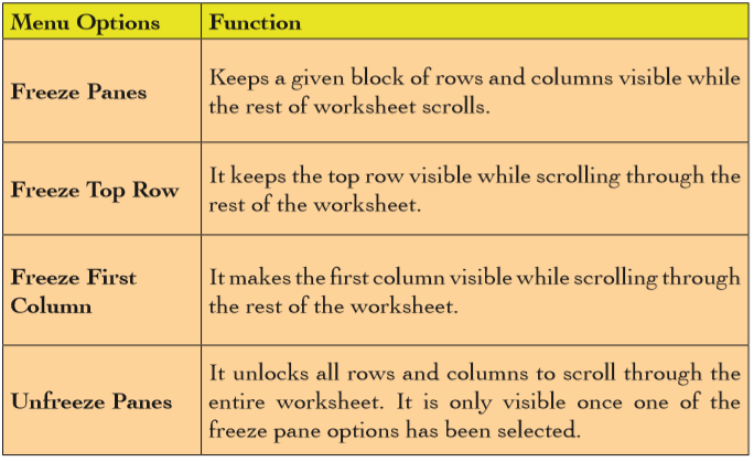
Table 5.1: Freeze menu options

5.2 Workbook View 

Microsoft Excel provides the following workbook views: Normal, Page break Preview, Page Layout, and Custom View. They are found in the View tab of the menu bar under the Workbook Views group. 

5.2.1 Normal 

It displays the worksheet in normal view. It is the default view. However, if the worksheet was displayed in another view, to change to normal view, select the Normal option from the Workbook Views group. The worksheet appears as shown in Figure 5.3. The keyboard shortcut is as follows: Long press ALT, press W then L.

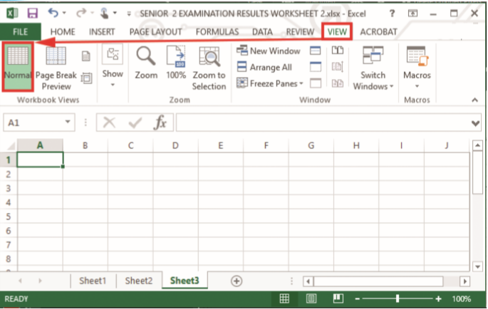
Figure 5.3:  The normal workbook view

5.2.2 Page Layout 

This view display the worksheet as it will appear on a printed page. It is used to view where pages begin, end and to view or insert footers or headers on the page.

It can only apply if no column or row has been frozen. To display a worksheet in page layout view, select the Page Layout option from the Workbook Views group.

The worksheet appears as shown in Figure 5.4. The keyboard shortcut is as follows:  Long press ALT, press W then P. 

5.2.3 Page Break Preview

 It is used to display a preview of where pages in a document will break when being printed. To display a worksheet in page break preview, select the Page Break Preview option from the Workbook Views group. The page numbers appear as water marks. The worksheet appears as shown in Figure 5.5. The keyboard shortcut is as follows: Long press ALT, press W then I.

Figure 5.4: The page layout workbook view

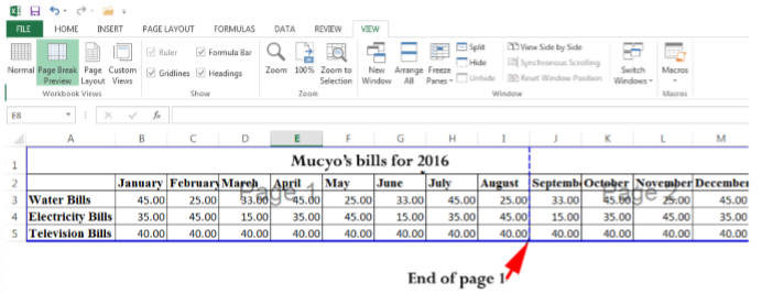
Figure 5.5: The page break workbook view 

5.2.4 Custom Views 

This is a flexible tool that can be used to view the same data in different ways, which is faster than manually changing the settings. This view can retain hidden columns and rows, some filters, zoom and print settings among others.

To create a customised view, do the following: 

(i) Select one of the above views then click on Custom Views option from the Workbook Views group. A dialog box appears as shown in Figure 5.6. The keyboard shortcut is as follows: Long press ALT, press W then C.

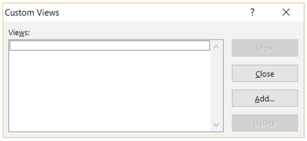
Figure 5.6: Adding a custom workbook view

(ii) Click Add… command. The Add View dialog box is displayed as shown in Figure 5.7. The keyboard shortcut is as follows: Long press ALT, press W then C, press Tab key to move to Add button then finally press Enter.

Figure 5.7: Naming a custom workbook view

(iii) Type the name of the view in the Name text box then click OK. 

(iv) To display a list of the created customised view, select the Custom Views option from the Workbook Views group. A dialog box appears as shown in Figure 5.8. To open a worksheet in an already created custom view, select the view from the Views list then click Show.

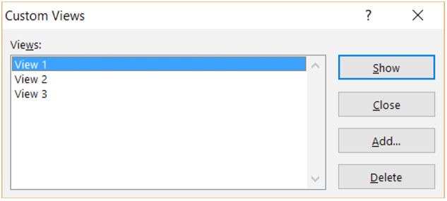
Figure 5.8: Viewing a workbook in a custom view

5.2.5 Split Worksheet 

Splitting a worksheet is necessary when all the information in it cannot be displayed in one view. This option divides the worksheet into four sections.  The user is able to scroll through a section of the worksheet while keeping other sections visible. The following are the steps followed to split a worksheet: 

(i) Position the cursor at the cell where the split should begin. For example, select Cell E10. 

(ii) Click on the View tab in the menu bar then select Split command on the ribbon from the Windows group. 

The worksheet is automatically split into four sections vertically at the left edge of the pointer and horizontally along the top edge as shown in Figure 5.9. 

The keyboard shortcut is as follows: Long press ALT, press W then S.

Figure 5.9: Splitting a worksheet

5.3 Sort and Filter 

Sort and filter commands are both used to enable the user access the required information faster. 

5.3.1 Sort

 Sorting refers to the process of arranging data in a predefined order. The order could either be ascending or descending. 

The ascending order is used when arranging data from the smallest to the largest while descending arranges the data from the largest to the smallest.  

The sorting feature is used for managing data in a large worksheet. To sort data, do the following: 

(i) Select the cell range containing the data to be sorted. 

(ii) Click on Data tab from the menu bar then select one of the sort option from the Sort & Filter group. 

(iii) To sort in ascending order, select the A to Z icon. To sort in descending order, select the Z to A icon. 

Figure 5.10 shows data that is sorted in ascending order (A to Z).  Figure 5.11 shows data that is sorted in descending order (Z to A). The keyboard shortcut is: Long press ALT, press A then SA and finally SD.

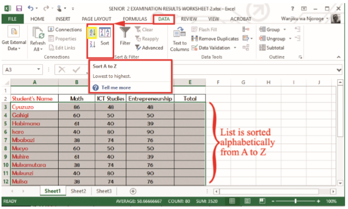
Figure 5.10: A worksheet sorted alphabetically in ascending order (A to Z)

Figure 5.11: A worksheet sorted alphabetically in descending order (Z to A)

(iv) To customise the sort, select the Sort icon. A dialog box is displayed as shown in Figure 5.12. Select the column to use under Sort by box, select the sort order in the Order box and the data to be sorted on the Sort On box then click OK. The keyboard shortcut is: Long press ALT, press A then SA and finally SS.

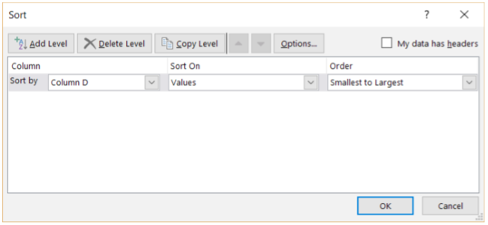
Figure 5.12: Customising the sorting order

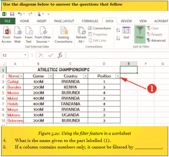
5.3.2 Filter 

It is done to only display records that meet a certain criteria. To filter data, do the following: 

(i) Select the cell range containing the data. 

(ii) Click on Data tab from the menu bar then select Filter command from the Sort & Filter group. The filtering controls are added to the worksheet headers automatically. Filtering can be done by number, text or colour. Figure 5.13 shows a window having filtering controls. The keyboard shortcut is: Long press ALT, press A then SA and finally T.

Figure 5.13: Filtering data

Filter by Number 

(i) Click the filter control of the column header to be filtered. Number Filters option is only activated if the column contains numbers. 

(ii) By default all the check boxes next to the numbers are marked (checked). Uncheck the check boxes which do not meet the desired criteria. Figure 5.14 shows Filter by numbers menu. 

Figure 5.14: Filtering by number 

(iii) Click OK. The worksheet will display all the records of people who are position 2. Figure 5.15 shows the filter results of the data. 

(iv) Select the filtering criteria display on the list box to the right, for example, select Equals ...

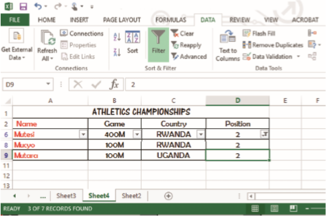
Figure 5.15: Filtered data

 Note: It is important to copy the data to another worksheet before filtering.

 Filter by Text 

(i) Click the filter control of the column header to be filtered. Text Filters option is only activated if the column contains text. 

(ii) By default all the check boxes are marked. Uncheck the check boxes which do not meet the desired criteria. Figure 5.16 shows a worksheet filtered by text. 

(iii) Click Ok. 

The worksheet will display all the records whose country of origin is Rwanda as shown in Figure 5.17.

Figure 5.16: Filtering by text

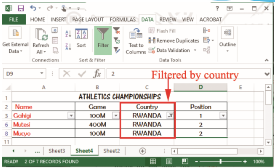
Figure 5.17: Filtered results

Filter by Colour 

(i) Click the filter control of the column header to be used to filter. 

(ii) Select Filters by Colour. This option is only activated if the cells in the worksheet have different colours. A side kick menu is displayed as shown in Figure 5.18. 

(iii) Select the colour to filter by from the side kick menu. 

(iv) Click OK to apply.

Figure 5.18: Filtering by colour

Custom filter 

This filter option enables user to specify with great accuracy the records that he or she desires to appear on the filtered list. To custom filter data, do the following: 

(i) Click on the filter control in the table header of the column to be filtered. 

(ii) Select Numbers Filters if the column has numbers and if the column has text entries, click Text Filters as shown in Figure 5.19.

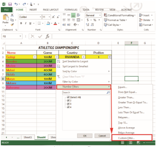
Figure 5.19: Custom filter menu

(iii) From the side kick menu, select Custom Filter… option. A dialog box appears as shown in Figure 5.20. 

For example, to show numbers equal to a certain amount, select Equals in the first box, then enter the number in the box in the adjacent box.

To filter by two conditions, enter filtering conditions in both sets of boxes, and select And for both conditions to be true, and Or for either of the conditions to be true. 

(iv) Then click OK.

Figure 5.20: Dialog box for custom filter

5.4 Definition of Key Words in this Unit

Revision Exercise 5