UNIT2: ADVANCED POWER POINT
POINT 2.0 INTRODUCTORY ACTIVITY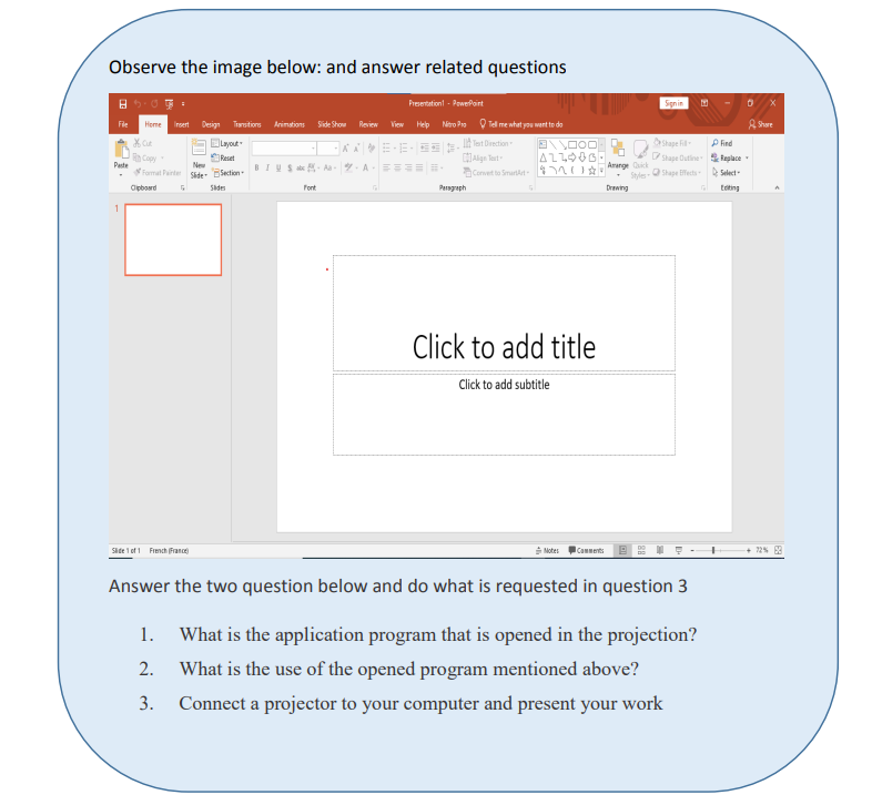 2.1. Create and Manage Presentations
 A presentation is an organized report or message prepared as a talk before anaudience, with the help of a computer program.A presentation software is a program used to create slide shows for presentation onscreen to an audience. Example of programs/software which can be used to createpresentations are the following:• Harvard Graphics,• Corel Presentations,• Lotus Freelance Graphics• Microsoft PowerPointThe role of Presentation applications is to help the presenter convey the messageeasily.Microsoft PowerPoint is presentation software commonly used when planning to givea talk as a presentation. The purpose of the talk may be to inform, create awareness,present strategies or to sell a product or service.A PowerPoint presentation is made by slides and it can be done on computer screenif the audience is very small and if the audience is large the computer can beconnected to a projector that projects the image onto a large screen or a wall.2.1.1 Starting PowerPoint PresentationTo start Microsoft PowerPoint 2013, 2016 & 2019 go through these steps:• Click to the start icon• Select and click on PowerPoint 2013 located on the startup menu• Click on one of the PowerPoint templates.In the new slide write the slide title and write the content in the appropriate zone.Here click on Blank Presentation. The PowerPoint screen appears as in the imagebelow:
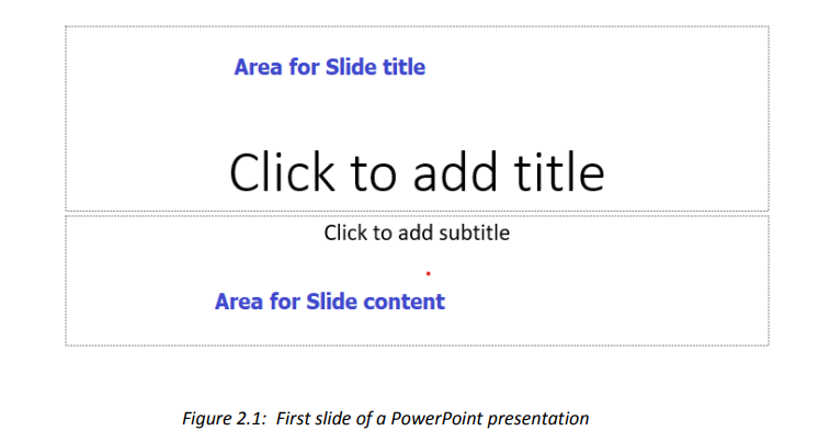
Resize the writing zones accordingly to make the title area small and the content area
bigger.
2.1.2 Creating and inserting a slide in a presentation
The opened PowerPoint presentation has now one slide and each slide has to have its
title set and have the content. Once this is finished a need to have more slides may
arise. To create a slide in an existing presentation, click on the Insert tab then click on
New Slide then choose the slide theme to apply.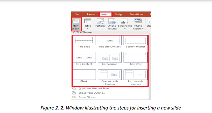
A new slide can also be inserted by selecting the slide behind which a new one is to
be inserted and hitting the Enter key.
The created presentation will be saved by clicking on the Save icon then choose thelocation where to save and specifying the name of the presentation.
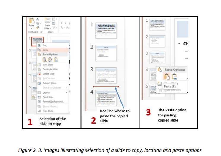
2.1.3 Copying a slide
A slide can be copied in the same presentation or copied to a new presentation in
order to avoid rewriting that presentation from scratch.
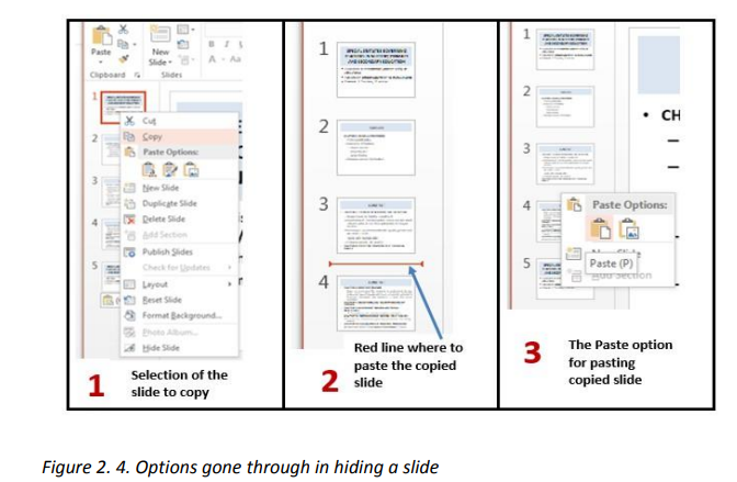
To copy a slide, do the following:
• Open the presentation containing the slide to copy
• In the left pane outlining the slides select the slide to copy
• Do a Right click and click on copy
• In the left pan click in the location where to put the copied slide so as to havea red line and do a right click and click Paste
2. 2. Managing Slides
Once the slides are created, one needs to know how to manipulate them by hiding
some slides, moving in slides, rearrange slides, delete some slides, dividing slides intosections, etc.
a. Hiding a slide
When a slide is not currently needed it can be hidden by selecting it then doing a Right
click and clicking on Hide Slide. The hidden slide will continue to appear in the slide
pane and can be opened by double clicking it but it won’t appear if the presentation
is opened in the Slide Show mode. To unhide the hidden slide go through the sameprocess.
b. Moving in slides
A slide that will be displayed on the computer screen or on the projector is the onewhich is selected.
In the Normal view to move from one slide to another use the Arrow keys found on
the keyboard. The Up key will move to the previous slide while the Down key will
move to the next slide. One can go to any slide without needing to serially go through
all slides by just clicking the slide to go to.
In the Slide Show view also use the same keys but not that the Escape Key can be used
to end the presentation in the Slide Show View mode and switch to the Normal view.Once the last slide is reached hitting the Down key will switch to the Normal View.
c. Rearranging slides
Slides are not stationary, they can be moved and rearranged making for example the
first slide be the third. To rearrange slides, select the slide, hold down the left buttonand move the slide by moving the mouse up or down.
d. Deleting slides
A slide that is no longer needed can be completely deleted by selecting it and hittingthe Delete key or selecting that slide, doing a Right click and clicking on Delete Slide.
e. Dividing slides into sections
Sections are subdivisions in a PowerPoint presentation slides used preferably for
bigger presentations that can be logically grouped. Slides in the same group should
be logically related so as to facilitate their understanding during presentation or while
reading them.
Putting slides into sections can also be done when slides are to be presented by
different people thus each person presents his/her section.
• Creating a section
To create a section in a PowerPoint presentation, do the following:1. Select in between the slides where to insert the section or the slide
behind which to insert the section
2. Do a right click and click on Add Section in the provided options
3. Rename the section by selecting it and clicking on Rename. The default
name of a section is Untitled Section.4. Write the new name and click Rename
A created section can be removed by selecting it, doing a right click and choosing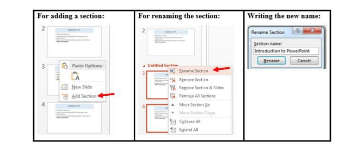
Remove Section. It can be moved by choosing the Move Section Up or Move Section
Down option.
2.3. Apply Design Themes and Format Background
a. Design theme
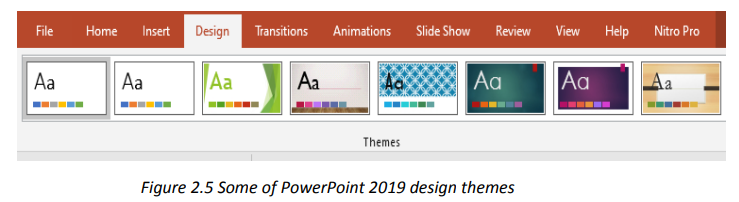
PowerPoint provides a variety of design themes which are predefined colors, fonts
and visuals that can be applied to slides to make them have a beautiful look withoutThe Themes gallery can be reached by clicking the DESIGN tab and themes willdoing a lot of formatting work.
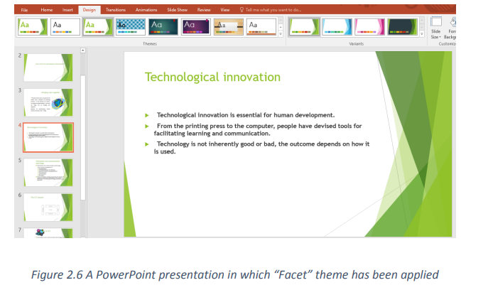
To apply a given theme to a presentation just open that presentation and select theimmediately be viewed.
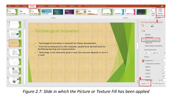
 b. Format background
desired Theme. In the image below the Theme “Facet” has been applied.
A background is an object which can be just a color, an image behind whatever text,To set a presentation’s background follow these steps:charts, images in a PowerPoint presentation.
• Open the presentation for which the background is to be set
• Under the DESIGN tab Click on Format Background
• Choose o n e o f t h e p r o v i d e d o p t i o n s and customize those optionsaccordingly
 a. Adding comment
2.4. Adding Notes and Comments, Inserting Header and Footer
In PowerPoint presentation, a comment is an explanation that is attached to a text
or an object on a slide, or to an entire slide.Step 2. Write the comments in the provided space as visible in the zone No 3 of theTo add a comment in a slide go through the following steps:
Step 1. On the Review tab, click New comment
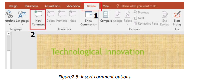
above image
Note: Comments can be added to a PowerPoint presentation by using a simpler
method of clicking at the Comment option located at the bottom middle of an openedPowerPoint window.
b. Adding notes
In a PowerPoint presentation Notes are words/text added to a presentation as
reference and only visible to the one presenting the slides. They serve as additional
information for the presenter that can be read for guidance as the presentation goesTo add notes to a presentation, do the following:on.
1. On the View menu, Click Normal
2. Select the thumbnail of the slide to add notes to
3. The notes pane will appear under the slide. Click where it says Click to addnotes and type whatever notes depending on your choice
Note: A simple way to add notes is to use the Notes option located at the bottom middle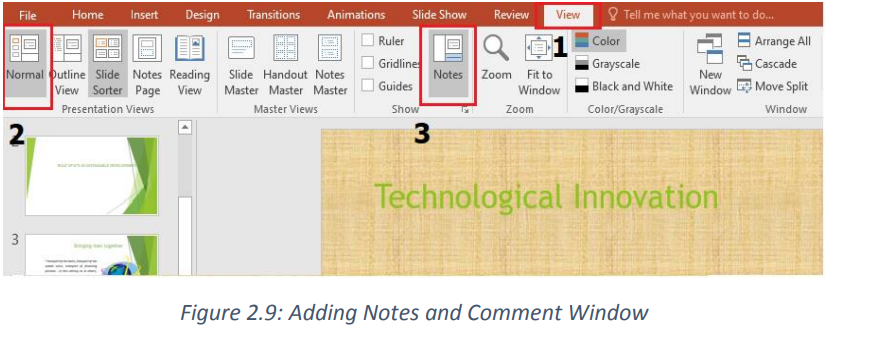
of an opened PowerPoint window
c. Insert header and footer
Header and footer in a presentation is the top and bottom parts of the slides. These
include the slide number, text footer and date.
To add a header or footer follow these steps:1. Click Insert then go to Header & Footer
2. In the box below Footer, type the text to use as footer such as the
presentation title
3. Check Date and time to add that to the slides
4. Check Slide number to add to the created slidesa. Inserting pictures5. Click on Apply or Apply to all if all slides are to have the same header orfooter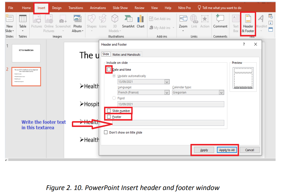
 2.5. Add Sound and Animation to Slides
 2.5.1. Animate text and picture in slidesIn PowerPoint, it is possible to animate text and objects such as clip art, shapes andpictures on the slide. Animation or movement on the slide can be used to draw theaudience’s attention to specific content or to make the slide easier to read.
To insert pictures in a slide, select the Insert tab, and then click the Pictures command.
Browse where the images are located and select one image and click Insert.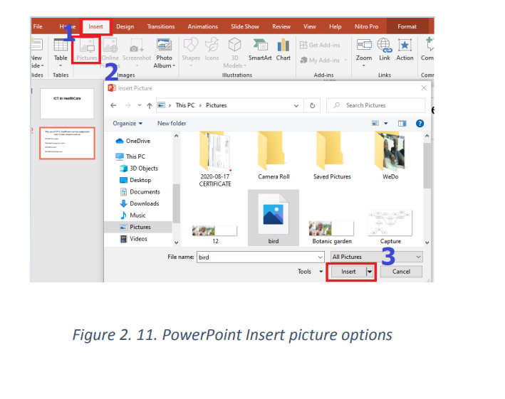 \
\
b. Animating a text or a picture.
When a text is written in a slide or an image inserted they can be animated using the
options available in PowerPoint. There are many types of animations available and
each is used for different reasons like making the message come to the screen in a
certain way (entrance animation) or bringing an emphasis to that message (emphasis
animations). The image below shows some of the animations available in PowerPoint2013.
For animating a text or an image do this: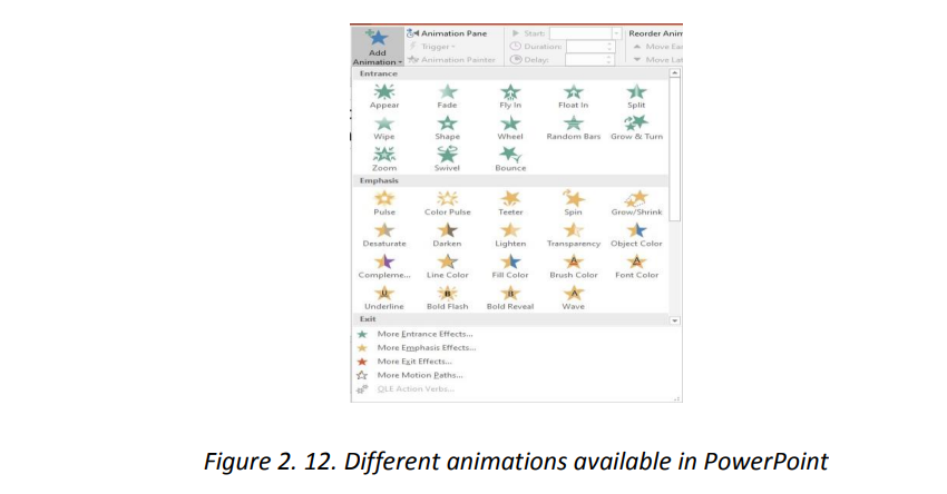
a. Select the text or picture to animate
b. In the Animation tab choose one of the available options like Float In, Split,
etc. The selected animation is immediately applied
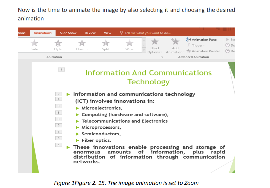
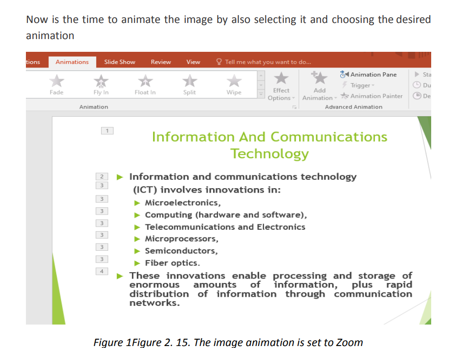
In the next images below the title has been animated with “Fly In” animation, the text
is animated with “Split” and the image is animated with “Zoom”. When the whole
slide is opened in Slide Show mode each element has its own animation which helps
attract more the attention of the audience.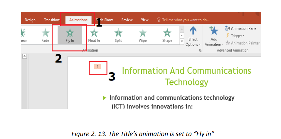 PowerPoint allows to use images, audio and video to have a greater visual impact.
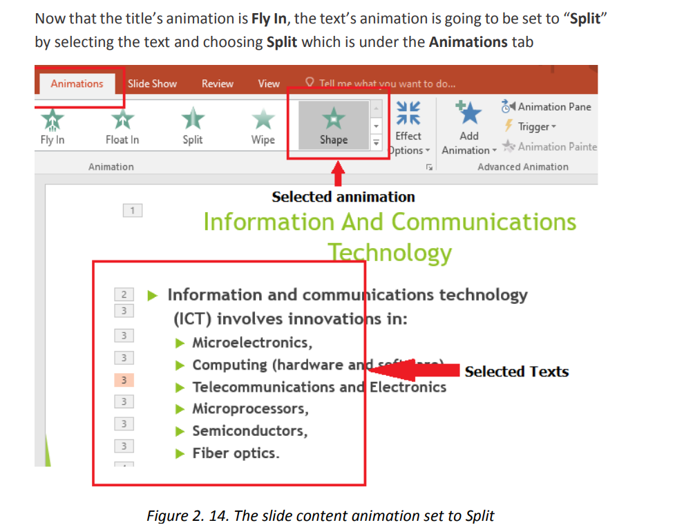
 Opening the above animated slide in Slide show mode will look like in thesequenced images below:
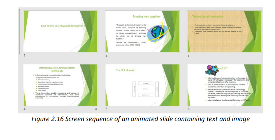 Interpretation :the above animated slide when opened in Slide view mode will show inthis way:a. A blank black screen will open and rapidly the black color will cede place tothe white background of a normal documentb. The text in the slide will come from left and right to meet in the middle c.The image will appear as a small image that will grow from the centerc. The title of the slide will appear from the bottom of the slide, slidingupwardB.1. Setting the delay of an animationThe default duration of a text or image animation can be changed to make theanimation slower or quicker. The delay cannot be greater than 59 seconds. To seta delay click on Animations tab and in the Timing group specify the duration and thedelay.
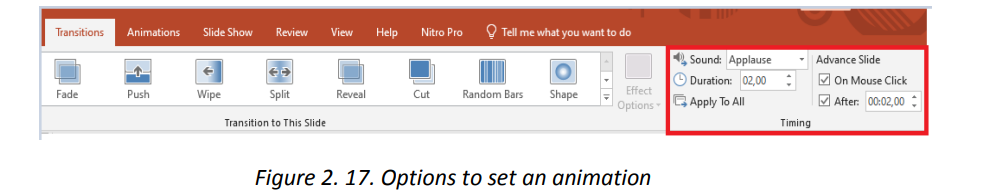 c. Customize animation effectsIt is possible to apply multiple animation effects to a text, an image or a picture. Whenworking with multiple animation effects, it helpsto work in the Animation Pane, wherea list of all the animation effects for the current slide is displayed.
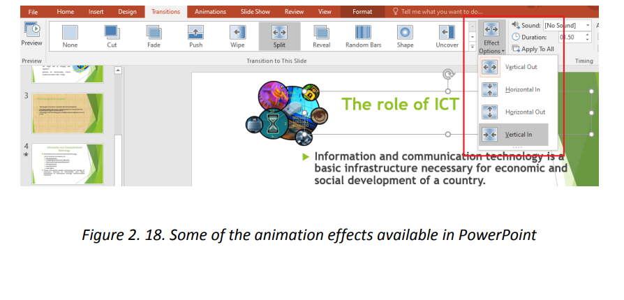
2.6 Add audio and Video Content to Slides
These visual and audio cues may also help a presenter be more improvisational andAnimation applied to text or objects in a presentation gives them sound or visualinteractive with the audience.
effects, including movement. It is possible to use animation to focus on important
points, to control the flow of information, and to increase viewer interest in aa. Inserting an audio or a videopresentation.
To insert an audio or a video do the following:
1. On the Insert tab click on Media
2. Choose the media to use which can be a video, an audio or a recording
which is taken using a computer
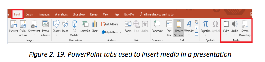
Browse the location where the audio or video to insert is located.
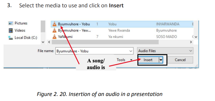 c. Inserting a screen capture
The slide where audio has been inserted will have a graphic as shown in below. Playusing the media buttons displayed.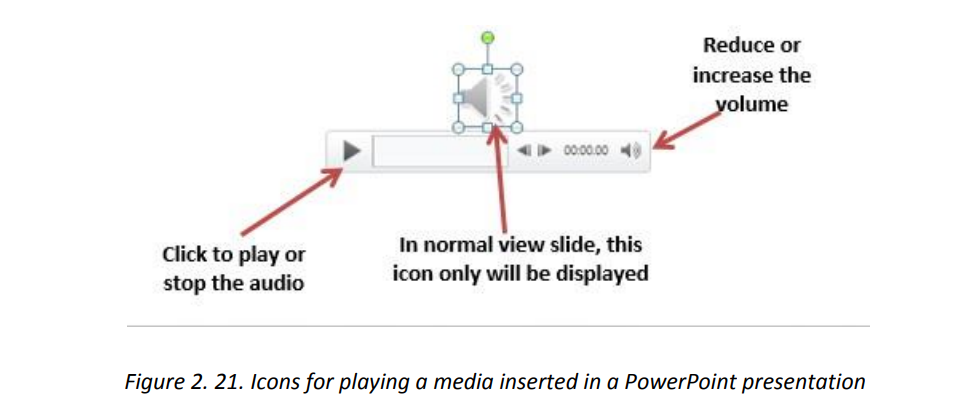 A media inserted in a PowerPoint presentation can have the role of providing moreclarification for efficient understanding, it can be the only content in the slide, it canbe a recording of the screen activity when for example one wants to show the steps todo a certain think using a computer. It can also be a readout of the slide’s text.b. Inserting a recordingA recording is taken using the computer microphone and is inserted much the sameway as other audio except that instead of browsing the audio to insert, the audio hasto be recorded. To insert a recording go through the following steps:1. Under the Insert tab click on Media2. Click on Audio then on Record Audio
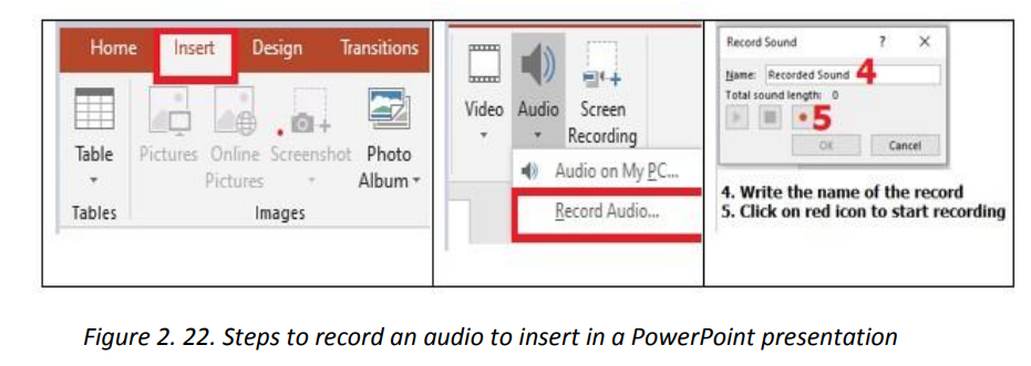 The recorded audio can be set to play as the slide is opened or to play whenclicked on. It can also be trimmed to fit in the desired time frame.To trim the recording:1. Click on the microphone icon then under the Audio tools go to Playback2. Click on Trim audio then on OK
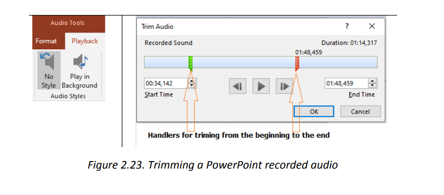
Capturing a screen can be very important for many reasons but the main is when you
want to make an instructional video that shows the steps that are being done on thescreen. This can be combined with capturing an audio describing what is being done.
Note: Thus, for future student teachers this functionality can prove very useful.
2. Choose among the available options in the dialog box that will appear, clickSteps to capture the screen:
1. Click on Insert then under the Media group go to Screen Recording
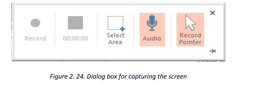
on Select Area to choose which portion of the screen to be recorded and click
on Record
3. To end the recording use the combination keys Window key with shift keyand Q
 2.7. Slide Transitions
 A slide transition is the visual effect that occurs when moving from one Slide to thenext during a presentation. Hereby one can control the speed, add sound, andcustomize the look of transition effects.a. Types of transitions:In PowerPoint 2019 there are two main slide transitions namely subtle, exciting anddynamic contentIn Subtle transition simple transitions are used to move from one slide to another, forExciting additional visual effects are used to catch the eye of the audience while forDynamic content will move only the placeholders, not the slides themselves.
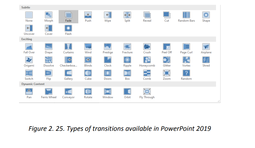 b. Using a transitionTo use the different transitions, do the following:• To select the text or image on which to apply the transitionOnce the transition has been set it can be modified by selecting the text having a• Click on the Transition tab then choose one of the transitions. In the imagebelow the chose n transition is “Dissolve”
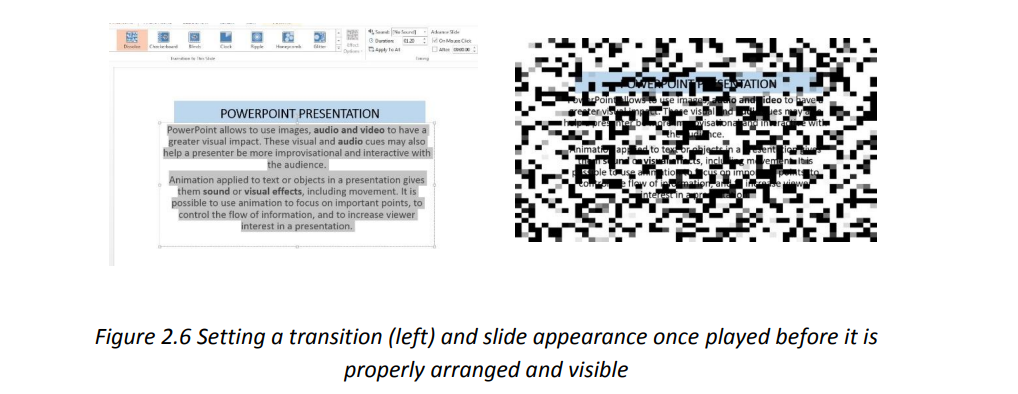
particular transition and choosing the new transition to apply. It can also be removedby choosing the None transition.
2.8 Presenting Using PowerPoint
Microsoft PowerPoint can add a visual dynamic to a business meetings and
presentations. The best way to share a PowerPoint presentation with a large group is
to project slides on screen using a digital projector connected to the computer’s videooutput.
a. Presenting using a projector
A projector is an output device that can take images generated by a computer andproduce them by projection onto a screen, wall or another surface.
A projector is connected to the computer through the VGA port but newprojectors and computers can be connected using the HDMI ports
Steps for connecting a laptop to a projector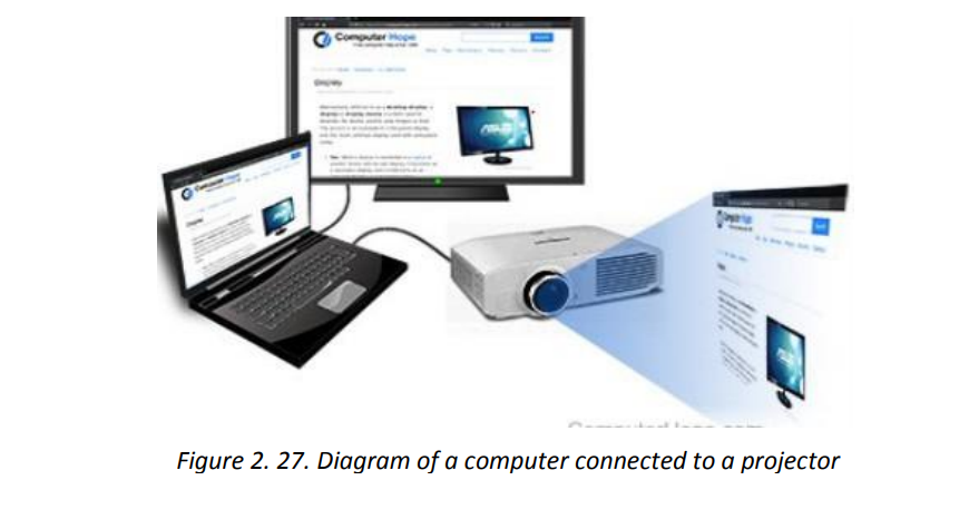
1. Make sure the laptop is turned off
2. Connect the video cable(VGA) from the laptop’s external video port to the
projector
3. Plug the projector into an electrical outlet and press the “power” button to
turn it ON.4. Turn on the laptop
There are different presentation modes while using a computer connected to a
projector. One can use the Projector only, duplicate (both the projector andcomputer), Extend and Disconnect the projector.
b. Printing and distributing handouts
A handout is a piece of printed information provided to the audience so as to give asummarized information on a given topic.
Handouts are distributed to an audience so as to help them follow the presentationand take some notes on what is being presented.
It is a good practice to give the presentations to the audience at the end of the sessionso as to review what was presented to them.
c. Conducting the presentation
When everything is in order; the projector is properly connected and working, the
handouts have been distributed and everyone is properly seated it is then time to startthe presentation.
For a presentation to be effective, the PowerPoint document have to have these
qualities:• Make the PowerPoint presentation short. Slides will contain short and concise
sentences which are bulleted,
• Highlight important points by using animations and transitions wisely not
randomly as these are used with a purpose like attracting attention on certain
section, notifying of the change in the topic, etc
• For long slides provide short partial synthesis to make the audience keep track
of what is so far presented
• Rehearse the presentation and use scripts and notes to help you not forget the
important points to mention
• Be polite and use appropriate language.