Physics

Unit 3: FORCED OSCILLATIONS AND RESONANCE OF A SYSTEM

Topic Area: OSCILLATIONS AND WAVES

Sub-Topic Area: Forced Oscillations and Resonance

Key unit competence: By the end of this unit I should be able to analyze the effects of forced oscillations on systems..

Unit Objectives:

By the end of this unit learners will be able to;

        ◊   Explain the concept of oscillating systems and relate it to the real life situations. 

        ◊ Solve equations of different types of damped oscillations and derive the expression for displacement for each. 

       ◊ explain resonance, state its conditions and explain its applications in everyday  life.

3.0 INTRODUCTION

In the conventional classification of oscillations by their mode of excitation, oscillations are called forced if an oscillator is subjected to an external periodic influence whose effect on the system can be expressed by a separate term, a periodic function of the time, in the differential equation of motion. We are interested in the response of the system to the periodic external force. The behaviour of oscillatory systems under periodic external forces is one of the most important topics in the theory of oscillations. A noteworthy distinctive characteristic of forced oscillations is the phenomen of resonance, in which a small periodic disturbing force can produce an extraordinarily large response in the oscillator. Resonance is found everywhere in physics and thus, a basic understanding of this fundamental problem is required.

Opening questions

Comment on the following situations by giving clear reasons on each;

    • A guitar string stops oscillating a few seconds after being plucked.

    • To keep a child moving on a swing, you must keep pushing.

3.1 DAMPED OSCILLATIONS.

Unless maintained by some source of energy, the amplitude of vibration of any oscillatory motion becomes progressively smaller and the motion is said to be damped. The majority of the oscillatory systems that we encounter in everyday life suffer this sort of irreversible energy loss while they are in motion due to frictional or viscous heat generation generally. We therefore expect oscillations in such systems to eventually be damped.

In everyday life we experience some damped oscillations like:

        (i) Damping due to the eddy current produced in the copper plate

 (ii) Damping due to the viscosity of the liquid

3.2 EQUATION OF DAMPED OSCILLATIONS

Consider a body of mass m attached to one end of a horizontal spring, the other end of which is attached to a fixed point. The body slides back and forth along a straight line, which we take as x-axis of a system of Cartesian coordinates and is subjected to forces all acting in x-direction (they may be positive or negative). The motion equations for constant mass are based on Newton’s second law which can be expressed in terms of derivatives. In all derivations assume that m is the mass of an oscillating object, b is the damping constant and k is the spring constant.

Where b is the damping constant and the negative sign means that damping force always opposes the direction of motion of the mass.

The spring itself stores the energy that is used to restore the position of the mass once released after being slightly displaced. The restoring force of the spring is directly proportional to the displacement.

Where k is the spring constant and the negative sign means that the restoring force opposes the direction of motion of the mass. With this restoring force and the resisting force of the spring, the resultant force on the mass is;

Equation 3-5 is the differential equation of damping.

3.3 THE SOLUTION OF EQUATION OF DAMPING

To solve the differential equation 3-5 (of damping), we try a solution of the form;

Substituting in equation 3-5,

Equation 3-6 is called the auxiliary quadratic equation of the differential equation. Solving this equation for y gives;
                                              

3.4 TYPES OF DAMPED OSCILLATIONS.

3.4.1 Under damping oscillation

This is also called a lightly damped oscillation. For this oscillation, the displacement keeps varying with time and oscillations keep dying away slowly and slowly. The vibrating system keeps passing its original position and more time is taken by it to come to rest. This is the case where the value of equation 3-8 under the square root is negative;

This means that damping constant b is small relative to mass m and spring constant k. So the solution of equation 3-7 becomes;

Equation 3-11 represents the displacement of under damped oscillation. From this equation it can be interpreted that the value of x decreases as time increase, but due to the trigonometric function of sine and cosine in bracket makes its graph on Fig.3-3 cross the horizontal axis so many times. Examples of slightly damped oscillations include

Acoustics

         (i) A percussion musical instrument (e.g. a drum) gives out a note whose intensity decreases with time. (slightly damped oscillations due to air resistance)

        (ii) The paper cone of a loud speaker vibrates, but is heavily damped so as to lose energy (sound energy) to the surrounding air.

3.4.2 Over damped oscillation

Over damping is also called excessive or heavy damping. In this oscillation, displacement decreases with increase in time but the vibrating system takes a longer time to come to rest. This is the case where the value of equation 3-8 under the square root is positive.

One extremely important thing to notice is that in this case the roots are both negative. You can see this by looking at equation 3-7 where the square root is less than b. The term under the square root is positive by assumption, so the roots are real.

The solution for expression 3-5 is;

Equation 3-12 represents the displacement of over damped. This equation is fully exponential and keeps the value of x decreasing towards zero in a quite long time Fig.3-3.

3.4.3 Critically damped oscillation

This is also called natural damping and is when there is an intermediate dissipating force and the system reaches equilibrium position as fast as possible without oscillating. This rapid return to the equilibrium position ( 0 =x ) reduces the motion to rest in a shortest possible time. This is the case where the term (of equation 3-8) under the square root is 0 and the characteristic polynomial has repeated roots, i.e. 

Now we use the roots to solve equation 3-5 in this case. We have only one exponential solution, so we need to multiply it by t to get the second solution.

Equation 3-14 represents the displacement of critically damped oscillation and shows that the displacement critically dies to zero in a short period of time as shown on Fig.3-3. It is possible to use the following values;

Where g    is the damping coefficient, w0  is the natural frequency and t    is the decay constant or the damping constant. Plotting equations 11, 12 and 14 on the same amplitude-time axes gives the general curve for damping oscillation as shown on Fig.3-3.

Examples of Critical damping

(a) Shock Absorber

It critically damps the suspension of the vehicle and so resists the setting up of vibrations which could make control difficult or cause damage. The viscous force exerted by the liquid contributes to this resistive force.

(b) Electrical Meters They are critically damped (i.e. dead-beat) oscillators so that the pointer moves quickly to the correct position without oscillation.

Analysis

• Calculate mean value for the time taken for the oscillator to come to rest for each radius of card.

• What is the uncertainty in the time taken to stop when the radius is 6 cm?

• Calculate this as a percentage of the mean value.

• What is the uncertainty in the time taken to stop when the radius is 8 cm?

• Calculate this as a percentage of the shortest time measurement at this radius.

• What is the uncertainty in the time taken to stop when the radius is 10 cm?

• Calculate this as a percentage of the longest time measurement at this radius.

• What type of error is responsible for the difference in the value of the time taken to come to rest?

• Calculate the area of the oscillator using . Write these values in the column provided.

• What is the precision in the radius of card measurements?

• Calculate the percentage uncertainty in the 7.0 cm measurement.

• What will be the percentage uncertainty in the value of the area?

• Write down the upper and lower limits of the area.

• Plot a graph of radius of Oscillator (on the y axis) against time taken to come to rest.

• Describe the graph you have plotted.

• What does your graph suggest about the relationship between the two variables?

• Plot a graph of area of Oscillator (on the y axis) against time taken to come to rest.

• Describe the graph you have plotted.

• What does your graph suggest about the relationship between these two variables?

• Complete the final columns of the table by calculating the additional area each card adds to the oscillator and the time period as a percentage of the undamped time taken to come to rest.

• Do you notice any patterns or trends?

• Plot a graph of additional area (y axis) against percentage of undamped time taken to come to rest.

• How are these variables linked?

• Theory states that damping will not affect the time period of the SHM system. How could you prove this using the experimental set up described above?

3.5  NATURAL FREQUENCY OF A VIBRATION AND FORCED OSCILLATION.

The natural frequency of an object is the frequency of oscillation when released. e.g. a pendulum. A forced oscillation is where an object is subjected to a force that causes it to oscillate at a different frequency than its natural frequency. e.g. holding the pendulum bob in your hand and moving it along its path either more slowly or more rapidly than its natural swing. Examples on forced oscillation include:

A: Barton’s Pendulum

The oscillation of one pendulum by application of external periodic force causes the other pendulums to oscillate as well due to the transfer of energy  through the suspension string. The pendulum having the same pendulum length and pendulum bob mass will have the same natural frequency as the original oscillating pendulum  and will oscillate at maximum amplitude due to being driven to oscillate at its natural frequency causing resonance to occur.

B: Hacksaw blade oscillator

This is another example of resonance in a driven system. If the peiod of oscillation of the driver is changed by increasing the length of thread supporting the moving mass, the hacksaw blade will vibrate at a different rate. if we get the driving frequency right the slave will reach the resonant frequency and vibrate widely. Moving the masses on the blade will have a similar effect.

3.6  EQUATION OF FORCED OSCILLATION AND ITS SOLUTION

These are vibrations that are driven by an external force. A simple example of forced vibrations is a child’s swing: as you push it, the amplitude increases. A loudspeaker is also an example of forced oscillations; it is made to vibrate by the force of the magnet and the current on the coil fixed in the speaker cone.

In addition to the restoring and damping forces in the spring, one may have an external force which keeps the oscillation going. This is called a driving force. In many cases, this force will be sinusoidal in time with maximum force F₀:

This equation differs from Equation 3-5 by the term on the right, which makes it in homogeneous.

The theory of linear differential equations tells us that any solution of the inhomogeneous equation added to any solution of the homogeneous equation will be the general solution.

We call the solution to the homogeneous equation the transient solution since for all values of b, the solution damps out to zero for times large relative to the damping time t.

We shall see that the solution of the inhomogeneous equation does not vanish and so we call it the steady state solution and denote it by It is this motion that we will now consider.

The driving term forces the general solution to be oscillatory. In addition, there will likely be a phase difference between the driving term and the response. The derivations below gives the general solution in terms of the amplitude A and phase angle

3.7  VARIATION OF FORCED FREQUENCY ON GRAPH AT AMPLITUDE CLOSE TO NATURAL FREQUENCY OF VIBRATION.

If an oscillating object is made to perform forced oscillations, closer is the frequency of force applied to the natural frequency, larger is the oscillation. However the amplitude rises and falls as the object will be assisted to oscillate for a short time and then the forces will oppose its motion for a short time. The graph shows the variation of the amplitude of the oscillations with time.

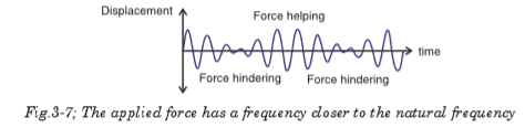
In figure 3.7, the applied force has a frequency closer to the natural

frequency. The amplitude of the oscillation has increased and there is time when the force helps and then hinders the oscillations.

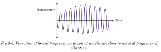
The largest amplitude is produced when the frequency of the applied force is the same as the natural frequency of the oscillation. When the energy input from the applied force is equal to the energy loss from the damping, the amplitude stops increasing.

3.8 RESONANCE

Resonance occurs when an object capable of oscillating, has a force applied to it with a frequency equal to its natural frequency of oscillation.

Each time the force is applied it transfers energy to the oscillation and increases its amplitude. A very large amplitude occurs after a short time. e.g. pushing a child on a swing. You record your pushes to have the same frequency as the swing. The windows rattle when a truck goes by if the frequency of the sound made by the truck’s engine is the same as the natural frequency of the glass when it is tapped.

The oscillator resonates when the amplitude in equation 3-22 is maximum, and this occurs if;

In these equations, g is the damping coefficient and w0 is the natural frequency.

3.9  APPLICATIONS AND EXAMPLES OF RESONANCE IN EVERYDAY LIFE

The phenomenon of resonance depends upon the whole functional form of the driving force and occurs over an extended interval of time rather than at some particular instant. Below are examples of resonance in different applications;

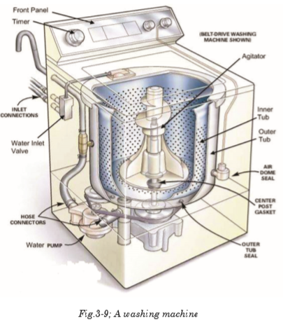
3.9.1 A washing machine

A washing machine may vibrate quite violently at particular speeds. In each case, resonance occurs when the frequency of a rotating part (motor, wheel, drum etc.) is equal to a natural frequency of vibration of the body of the machine. Resonance can build up vibrations of large amplitude.

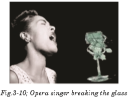
3.9.2 Breaking the glass using voice

You must have heard the story of an opera singer who could shatter a glass by singing a note at its natural frequency. The singer sends out a signal of varying frequencies and amplitudes that makes the glass vibrate. At a certain frequency, the amplitude of these vibrations becomes maximum and the glasss fails to support it and breaks it. This scenarion is shown on Fig.3-10 below.

3.9.3 Breaking the bridge

The wind ,blowing in gusts, once caused a suspension bridge to sway with increasing amplitude until it reached a point where the structure was overstressed and the bridge collapsed. This is caused by the oscillations of the bridge that keep varying depending on the strength of the wind. At a certain level, the amplitude of oscillation becomes maximum and develops crack on it and suddenly breaks.

3.9.4 Musical instruments

Wind instruments such as flute, clarinet, trumpet etc. depend on the idea of resonance. Longitudinal pressure waves can be set up in the air inside the instrument. The column of air has its own natural frequencies at which it can vibrate. When we blow, we use the mouthpiece to start some vibrations. Those which happen to match exactly the natural frequencies of the instrument are picked out and magnified.

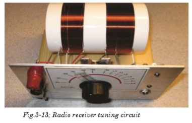
3.9.5 Tuning circuit

The another example of useful resonance is the tuning circuit on a radio set. Radio waves of all frequencies strike the aerial and only the one which is required must be picked out. This is done by having a capacitance inductance combination which resonates to the frequency of the required wave. The capacitance is variable; by altering its value other frequencies can be obtained.

3.9.6 Microwave Ovens

Microwave ovens use resonance. The frequency of microwaves almost equals the natural frequency of vibration of a water molecule. This makes the water molecules in food to resonate. This means they take in energy from the microwaves and so they get hotter. This heat conducts and cooks the food.

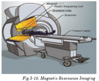
3.9.7 Magnetic Resonance Imaging (MRI)

The picture showing the insides of the body was produced using magnetic resonance imaging (MRI). Our bodies contain a lot of hydrogen, mostly in water. The proton in a hydrogen spins. A spinning charged particle has a magnetic field, so the protons act like small magnets. These are normally aligned in random directions. Placing a patient in a strong magnetic field keeps these mini magnets align almost in line. Their field axis just rotates like a spinning top. This is called processing.

3.10 EFFECT OF RESONANCE ON A SYSTEM

     ◊  Vibrations at resonance can cause bursting of the blood vessel.

     ◊  In a car crash a passenger may be injured because their chest is thrown against the seat belt.

     ◊  The vibration of kinetic energy from the wave resonates through the rock face and causes cracks.

     ◊  It is also used in a guitar and other musical instruments to     give loud notes.

     ◊  Microphones and diaphragm in the telephone resonate due to radio waves hitting them.

     ◊  Hearing occurs when eardrum resonates to sound waves hitting it.

     ◊  Soldiers do not march in time across bridges to avoid resonance     and large amplitude vibrations. Failure to do so caused the loss of   over two hundred French infantry men in 1850.

     ◊  If the keys on a piano are pushed down gently enough it is possible to avoid playing any notes. With the keys held down, if any loud noise happens in the room (e,g. Somebody shouting), then some of the notes    held down will start to sound.

     ◊  An opera singer claims to be able to break a wine glass by loudly singing a note of a particular frequency.

EXAMPLES

1. Solve the following initial value problem and determine the natural frequency, amplitude and phase angle of the solution.

2. Solve the following initial value problem. For each problem, determine whether the system is under, over, or critically damped: