Economics

Key unit competence: By the end of this course unit, you will be able to describe economic phenomenon using mathematical tools

4.1 EQUATIONS IN ECONOMICS
4.1.1 Linear equations and linear graphs
(a) Linear Equations

Activity 4.1
The table below shows the sales revenues and advertising expenditures of Quality Supermarket.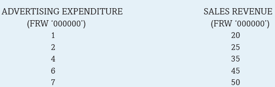

In groups of five,
(a) Explain the relationship between advertising and sales as reflected in the above table.
(b) Determine the sales revenue generated at FRW 9 million and FRW 10 million levels of advertising.
Give reasons for your answer.

Facts
From the table given in the question above, we can see that the supermarket makes more sales as a result of higher advertising. This shows a relationship between advertising expenditure and sales revenue. We can say that the higher the advertising expenditure, the higher the sales by the supermarket.

Sales revenue therefore depends on advertising. In this case we call sales revenue a dependent variable while advertising an independent variable. This is because sales depend on advertising. Advertising is independent because it is not being affected by sales or any other factor. We will come across such cases in Economics and Mathematics more often.

This relationship can be expressed as an equation, as follows:
Y =a +b x, Where
y is the dependent variable (sales revenue in this case).
x is the independent variable (advertising in this case).
a is a constant figure. It represents the amount sold without any form (at zero level) of advertising i.e. If x=0, y =a. In the case on page 41, Activity 4.1, sales made without advertising are lower than 20,000,000 FRW. (Assuming advertising begins at 1 million FRW).
b is a coefficient. It shows how much y will change every time x changes by one unit.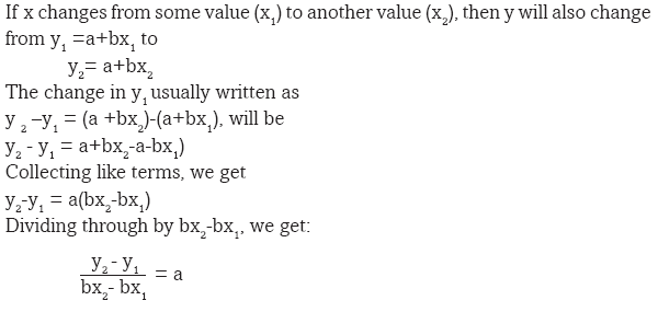

The above case is an example of a linear equation. Linear equations are referred to as first degree polynomials.

From the table above, following advertising and sales figures of Quality Supermarket, we can see that sales increase by 5 million from 1 million advertising expenditure.

Therefore, at zero advertising expenditure, sales would be 20m-5m=15 million.
Therefore our equation, y =a+bx
Would be y= 15+5x.

Given this equation, we can be able to find out:
The amount of sales arising from a given expenditure in advertising.
The amount of advertising necessary to generate a desired amount of sales revenue.

Example 1
The sales revenue generated by 10 million advertising expenditure would be:

Y=15 +(5x10)
=15 +50 =65m

Example 2
If Quality Supermarket targeted sales revenue of 75 million FRW, determine the advertising expenditure that it would have to incur.

Solution
y = a + b x
75 =15+5x
60=5x
X=12
Therefore the amount of advertising needed to yield 75 million FRW would be 12 million FRW.

(b) Sketching linear graphs
The data from the table on sales and advertising for Quality Supermarket (Activity 4.1) can be plotted on a graph.

The graph has two sides called axes. The upright side (side having an arrow pointing up) represents the vertical axis. The bottom side (side having an arrow pointing to the right) represents the horizontal axis.

The values of the dependent variable (sales revenue in this case) will be represented on the horizontal axis. The values of the independent variable (advertising expenditure in this case) will be represented on the vertical axis.

Values on the horizontal axis increase as we move to the right, from the point of origin. Similarly, values on the vertical axis increase as we move upwards, from the origin.

In the case of Quality Supermarket, y stands for sales while x stands for advertising.

Each row of the table gives us a pair of numbers, or a combination of x and y.
We have 1 and 20, 2 and 25 and so on.

These pairs are written as (1, 20), (2, 25)...
To plot the pair (x,y) begin at the origin where the two axes meet. Count rightward x units on the horizontal axis and then count y units above this level, parallel to the vertical axis. Mark this spot. Continue with the process for the different pairs of x and y. After identifying and marking all the pairs, then connect the pairs. This can be done by drawing a line that passes through all the points.

Using the example of Quality Supermarket, all the pairs are along the same straight line.

From our equation y= a+bx, ‘a’ represents the point at which the line joining the paired points cross the dependent line. In economical and mathematical terms, we say the derived line intercepts the vertical axis at point a. ‘a’ is therefore referred to as the vertical or y intercept.
‘b’ on the other hand is the slope of the line.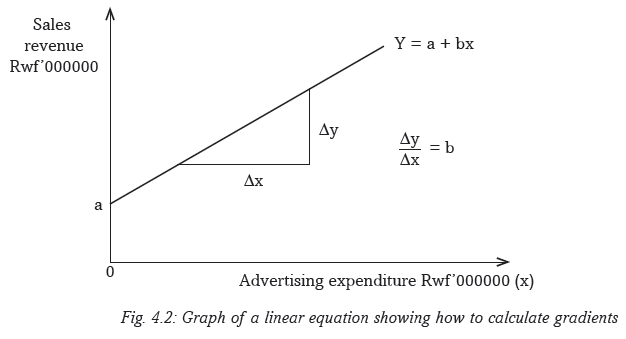

The slope ‘b’ tells us the rate at which the y variable changes with a unit change in x.

Recall
What do we call ‘b’ in Mathematics?

Note that ‘a’ has no effect on the slope of the graph.
Let us point out that the value of ‘a’ can be either positive, negative or zero.
When the value of ‘a’ is positive, the graph will intercept the vertical axis above the origin.
When the value of ‘a’ is negative, the graph will intercept the vertical axis below the origin.
When the value of ‘a’ is zero, the graph will intercept the axis at the origin.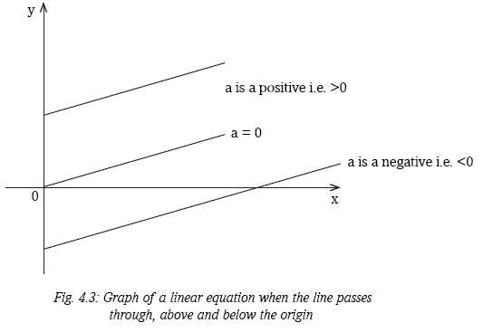

Examples of linear equations in economics
There are several types or examples of linear equations as used in Economics.
The main examples are:
1. The production possibility frontier; a graph that shows combinations of goods and services that can be produced with a given level of resources.
2. The demand function; an equation showing the various quantities of goods purchased by customers at given prices.
3. The supply function; an equation showing the various quantities of goods brought to the market by suppliers at a given market price.
4. Isocost line; a graph showing different combinations of labour and capital that can be purchased by a given firm.

The demand curve

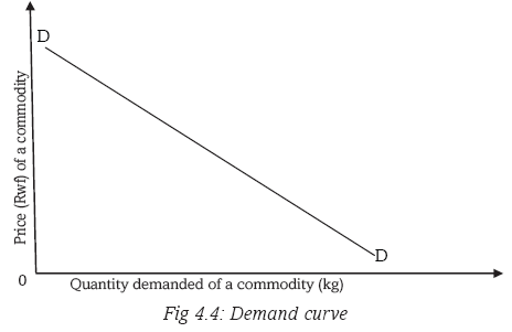
The demand curve shows the relationship between the quantity demanded of a commodity and the price of that commodity. This is a negative slope. It shows that an increase in the independent variable (price) leads to a decrease in the dependent variable (quantity demanded).

The supply curve

The supply curve shows the relationship between the quantity supplied of a commodity to the market by suppliers and the price of the commodity. This has a positive slope. It shows that both the price (the independent variable) and quantity supplied (the dependent variable) change in the same direction.

4.1.2 Non linear equations and non linear graphs
Non-linear algebraic equations are polynomial equations of a degree that is greater than one. They are mathematical relationships that describe non linear graphs. They take various types. For instance, we have the following main non- linear equations:
   (a) Polynomials
   (b) Logarithmic equations
   (c) Conic equations
   (d) Exponential equations

Activity 4.2
The following tables show the changes in variable Y as a result of changes in variable X.

Table 1

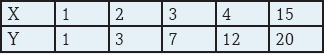
Table 2

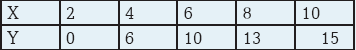
(a) Sketch the information given in Tables 1 and 2 in their respective charts.
(b) In groups, discuss the relationship between the two variables as revealed by the charts.

4.1.2.1 Features of non linear equations
1. In non linear equations, the independent variable has a certain power to it. If we have y as the dependent variable and x as the independent variable, the relationship could be: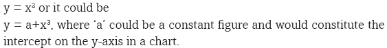

2. The features of non linear equations vary, depending on the gradient or slope of the curve.
3. Where there is one independent variable whose power is greater than one,

   the dependent variable will increase at an increasing rate as the power of the independent variable rises.

For example if

The graph from the equation above would curve upwards. As y increases at a faster rate than x. This is shown below.

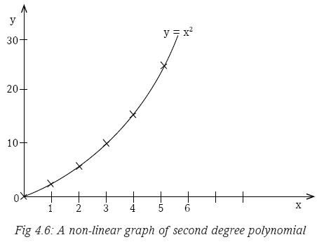
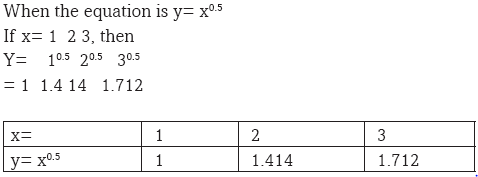
4. Where the power of the independent variable (x) lies between 0 and 1, then the value of y will also be increasing as x increases.

Example

5 Where the power of x is negative with the value of x being positive, the graph derived would slope downwards. This graph would take a convex curve shape.
In this case, the dependent variable increases as the independent variable (x) decreases.

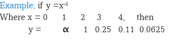
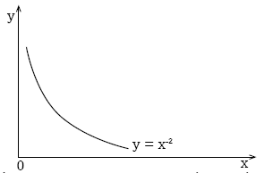
Fig. 4.8: A non-linear graph where the power is negative (less than zero)

4.1.3 Simultaneous equations

Specific objectives
By the end of this sub-unit, you should be able to:
(a) Identify different methods of solving simultaneous linear equations.
(b) Solve simultaneous linear equations.

Activity 4.3

The following table shows the demand and supply conditions relative to the change in the price of commodity x.

(a) In groups of five, discuss the relationship between:
    (i) The price and the demand for the commodity.
   (ii) The price and the supply for the commodity.
(b) Sketch the demand and supply relationships in a chart.

4.1.3.1 Necessary conditions for simultaneous equations

These conditions include that:
    (i) There should be more than one functional relationship, between a set of specified variables

such as x and y or q and p.
   (ii) That all the functional relationships are in linear form.

    It is then that we try to find the value of the unknown variables in the equations.
In the case where we have only two variables in the equations, it is then possible to subject the equations to graphical solutions.
Simultaneous equations can be solved using various methods.

4.1.3.2 Methods used in solving simultaneous equations
a) The substitution method

This method entails representing one unknown in terms of the other unknown.
Example
Find the values of x and y in the following equations using the substitution method.
20 x + 6 y =500…………….. (i)
10x – 2 y = 200……….......... (ii)

If we arrange equation (ii) so as to define or represent y in terms of x, we get:
10x - 200=2y
Dividing through by 2, we get:
5x-100 =y

We then substitute the new value of y (obtained in equation (ii)) in equation (i) as follows:
20x +6y=500 .....(i) now becomes
20x +6(5x-100) =500 ........(iii)
On opening the brackets, we get:
20x +30x -600=500
On collecting like terms, we get:
50x=1100
x=22

We would then substitute the value of x in equation (ii) to get:
220-2y=200
220=200 +27
20= 2y
y =10

b) Row operation method
We can also use the row operation to get the same result. Using the above example,
Where 20x + 6y =500 and ………..(i)
10x – 2 y =200……….. (ii)
Multiplying equation (ii) by 3, we get:
30x - 6y=600………… (iii)
Adding equation (iii) to equation (i), we get
50x =1100
x =22

We then substitute for x in any of the equations to get y=10.
We can apply the concept to solve for demand and supply relationships, when given the demand and supply functions.

Note: Unlike in the usual linear relationship between the dependent and independent variables, in this case, our relationships are expressed in a reversed manner. For example, p=f(q) and not q=f(p). The dependent variable is on the horizontal axis while the independent variable is on the vertical axis. This is because price is normally measured on the vertical axis. The principle is the same and the idea is to get the true relationship of the variables.

Therefore, if we are given the following demand and supply equations:
p=840—0.4q as a demand schedule
And p =120+0.8 q as a supply schedule,
We can solve for both p and q
(i) Multiplying demand schedule by 2, we get:
2P+1680 -0.8q
(ii) Adding the new demand schedule to the supply schedule, we get:
3P=1800
P=600

(iii) Substituting for P in any of the equations, we get:
600=120+0.8q
0.8q=480
8 q =4800
q=600

We could also use the equation method to solve for the demand and supply quantities such that:
840-0.4q=120+0.8q
720+1.2 q
q=600

Substituting for q in any of the two equations, we get:
P=600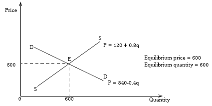

Fig. 4.9: Graph showing equilibrium price and equilibrium quantity

Activity 4.4
Taking P for price and the other unknown for quantity, solve the simultaneous linear equations. They represent the various demand and supply functions we come across in our daily lives. Illustrate your findings on graphs. Make class presentations.

Group A
1. Q = 3P + 2, Qs = 2 - P
2. 3P + 7Q = 10, 4P - Q = 3
3. 5P + 10Q = 10, 2P - Q = 1
4. 2P + Q = 7, 3P + Q = 10

Group B
5. 5P + 3Y = 7, 4P - 5Y = 3
6. 4P + 6Q = -13, 3P - 5Q = 14
7. 6P + 3Q = 1, 4P - 2Q = 2
8. 3P + 5Q = 12, 6P - 4Q = 3

Group C
9. 6P + 3Q = 2P + Q = 1
10. 2P + Q = 7, 4P + Q = 11
11. 5P + 7Q = 12, 6P - 3Q = 3
12. 2P + 3Z = 2, 6P - 12Z = 13

Note: You can use any of the above methods earlier learned, or any of these methods.
(a) Elimination method
(b) Matrix method
(c) Graphical method
(d) Crammer’s method
(e) Inverse method

Other examples of non linear graphs in Economics
a) Average cost curve

The average cost curve (AC) shows the relationship between the output produced and the variable cost spent on producing each unit of this output.

b) The average product curve

The average product curve (AP) shows the relationship between the variable factor employed and the output produced from each unit of the variable factor.

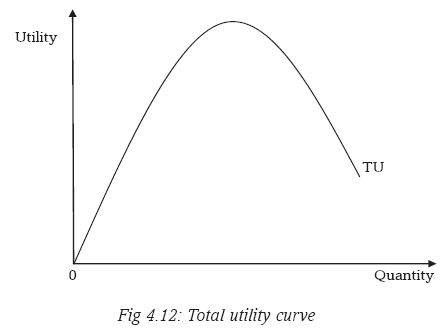
c) Total utility curve

4.1.4 Differential equations and graphs

A differential equation is a mathematical equation that relates some function with its derivatives. Functions are usually represented by physical quantities. Derivatives represent the rates at which the physical quantities change. Thus differential equations define the relationship between the two.
Differential equations have types. For instance:
• Ordinary differential equations.
• Partial differential equations.

An ordinary differential equation (ODE) is an equation that contain a function of one independent variable and its derivative. These equations can either be linear or non linear. For instance,

A partial differential equation (PDE) is a differential equation that contains unknown multivariable functions and their partial derivatives. These equations are used to formulate problems involving functions of several variables. For instance,
y = 2x∂x + 8

4.1.4.1 Linear and non-linear differential equations
Maxima and minima points

Maximum (maxima) and minimum (minima) points have an important application in Economics.

Economic application

Example
Given A total revenue function
TR = 120Q-2.5Q2
Find marginal revenue function.

The derivative is denoted dy or f(x) and is given by dividing the change in y
                                         dx
variable by change in change in x variable.

Rules of differentiation (Elementary level/basic level)
1. Constant rule
if given a function y=k where k is a constant, then

2. Power function rule

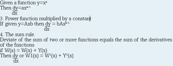
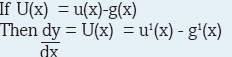
5. The difference rule
The derivative of the difference of two or more functions equals the difference of the derivatives of the functions.

The derivative of the difference of two or more functions equals the difference of the derivatives of the functions.

Both ordinary and partial differential equations are broadly classified as linear and non linear equations. A differential equation is linear if and only if the unknown function and its derivative appears to be power 1. Otherwise it is non linear. For instance,

dy = 8 is a linear differential equation.
dx
y = 8x + C is a non linear differential equation.

In Economics, differential equations are essential in computing marginal values of a nature

Marginal revenue 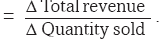 This is the additional revenue accruing to the firm from the sale of an additional unit of output.

Marginal product 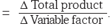This is the additional/extra units of output that are derived from the employment of an additional unit of a variable factor.

Marginal cost  This is the additional cost of producing and extra unit of output.

4.2 FRACTIONS IN ECONOMICS

Specific Objectives
By the end of this sub - unit, you should be able to:
(a) Express the ratios of quantities of various items or variables in Economics.
(b) Determine the proportions of given quantities of an item relative to the whole amount of the item.
(c) Calculate the percentages of given quantities of economic variables.
(d) Derive the reciprocals of given numbers of economic variables.
(e) Calculate averages and index numbers from given economic data.
(f) Derive absolute values from given values.

Activity 4.6
The annual budget for country X was 550b US $. It was allocated as shown below.

                   Sectoral budgetary allocation

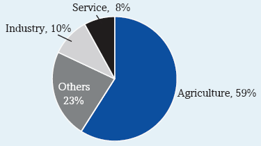
Use the figures above to answer the questions that follow.
(a) Determine how much was allocated to the service sector.
(b) Express the agricultural allocation in billions as a ratio of the total budget.
(c) What fraction of the budget went to other sectors?
(d) What proportion of the 550b $ was allocated to the industrial sector?
(e) Agriculture was allocated a lion’s share of the budget. In your own view, why do you think could have been the reason for this.
(f) Identify the sectors that may be included in the ‘others’.
(g) Would you take the above to be a good budgetary allocation to suit your country? Support your answer.

Facts
Fractions are numbers that are expressed with numerators and denominators. The numerator represents part of a whole unit. In a class for instance, if you are forty students and half of them are boys, then we will say 20 out of 40 or half the class are boys.

Activity 4.7
Simon, a large scale farmer, has the following livestock on his farm:
1) 50 dairy cattle, 40 of which are currently being milked;
2) 100 beef cattle, 60 of which are cows;
3) 200 goats, 40 of which are he- goats.

Required:
(a) Determine:
i) The total number of livestock that the farmer has.
ii) The total number of male livestock.
iii) The total number of cattle.
(b) In groups, discuss the reasons that may have made Simon to:
i) Keep more goats than cattle on his farm.
ii) Keep more beef cattle than dairy cattle.

4.2.1 Ratios

Activity 4.8
In groups of five, work out the following:
(a) For a sugar-producing firm, the ratio of total fixed costs to total costs is 4:10. Determine value of its total variable costs if it spends 40 millions FRW as fixed costs.
(b) In a class, the ratio of girls to boys is 7:3 and the ratio of day scholars to borders (both girls and boys) is 2:8. If the number of boarders is 400 students, determine the number of and girls in this class.
(b) Christine works with Rwanda Environment Authority and consumes 400000 FRW of her net salary per month. If the ratio of her savings to net salary is 6:20, determine how much she saves.

Facts
The question that we need to answer here is, what is a ratio?
Simply stated, a ratio is a number representing a comparison between two things that are in a way related. For example, if we look at the farm of Simon in the activity given at the beginning of this unit, we see that there are 40 dairy cattle that are being milked out of 50. Therefore, the number of dairy cattle that is not being milked is 10. From this information, we can derive the following ratios:

i) The ratio of the number of cows being milked to the total number of dairy cattle is 40:50. This can also be expressed in the form of a fraction as 40/50.
ii) The ratio of the dairy cattle that are not being milked to those that are being milked is 10:40. This ratio can also be expressed as 10/40.
iii) The ratio of the number of the cattle that are not being milked to the total number of the dairy cattle is 10:50. This ratio can also be expressed as 10/50.
The ratio derived can be further simplified to the lowest form possible such that in i), we would get a ratio of 4:5, in ii) we get 1:4, while in iii), we get 1:5.

Recall
From the information given in the activity at the beginning of this unit, determine:
(a) The ratio of beef cattle to the total number of cattle in the farm.
(b) The ratio of bulls to cows in the case of the case of the beef cattle in the farm.
(c) The ratio of cattle to goats in the farm.
(d) The ratio of the hegoats to the shegoats.

4.2.2 Proportions
A proportion is the quantity of a given item that is part of the whole amount or number of that item. For example, supposing Juma who earns $200 a month saves $50 every month. Then the proportion of income saved by Juma is 50 out of 200, or 5 out 20 or further simplified to 1 out 4. We can therefore say that out of every $1 that Juma earns, he saves $0.25. This is the marginal rate of saving by Juma.

At the macro level, we could also be able to determine the proportion of the total budget that the Government spends on either education or on health or on armament. In this way, we could be able to gauge whether resources are being optimally allocated or not.

Activity 4.9
Visit the National Institute of Statistics Rwanda website [statistics/] and write short notes after discussion on the following:
(a) Contribution of each of the following sector to cross domestic product (in percentage) of ratio.
- Agriculture
- Industry
- Services

(b) Percentage of population living below poverty line.
(c) Economic growth for year 2013, 2014.
(d) Population growth, fertility rates.
(e) Gender composition of total population.
(f) Literacy levels.

4.2.3 Percentages

Activity 4.10
In groups of five, work out the following:
(a) Umuhoza Patience spent 20000 FRW of her monthly salary on transport. Express this as a percentage of her salary if she earns 250000 FRW monthly.
(b) In a class of 40 students, 25 are girls. Express the number of boys as a percentage of the whole class.
(c) Given that the price of commodity X increased from 500 FRW to 850 FRW per unit, what is the percentage change in price of commodity X?
(d) Twahirwa John and Muhoza Patience work for KSW Ltd. Their salaries were increased last month. Twahirwa now earns 200000 FRW up from 100000 FRW. On the other hand, Muhoza now earns 500000 FRW up from 370000 FRW. Compare their increments and discuss who got a bigger increase. Explain your answer.

Percentage is a way of expressing the magnitude of a given quantity in relation to 100 such quantities. It shows the amount, number or rate of something as part of a total of 100.

In the case of the firm of Simon in Activity 4.7 given at the beginning of this unit, we saw that the ratio of the dairy cattle being milked to the total number of dairy cattle was 4:5 or 4/5. This is because, out of the total 50 dairy cattle, 40 were being milked. To find the percentage of these cattle being milked to the total number, we would divide 40 by 50 and then multiply by 100 for example 40 or 40/50 then multiply the result by 100. This would give us a figure of 80. We would then say that 80 percent of the dairy cattle on the farm are being milked. This is written as 80%.

This concept of percentages is of great significance in economic analysis. This is because it gives a quick glimpse of the magnitude of a given variable in relation to a total. For example, if we are told that the youth of country X constitute 60% of the total population of that country, this gives us an immediate and clear idea of the magnitude of the population problem.

At the work place, it would also be more meaningful to talk of the number of female employees in percentage terms as a way of determining the extent of equity in employment. It is also more meaningful to the common person when changes in certain economic parameters are expressed in terms of percentages rather than in absolute terms. We are therefore more comfortable when told of a 10% increase in the cost of living or a 20% increase in the level of wages.

In microeconomics, percentage is mainly used to determine the degree of changes in:
• Price
• Quantity
• Elasticity
• Costs
• Profit

In macroeconomics, calculation of percentages is mainly done to determine macroeconomic indicators like:
• Gross domestic growth (GDP)
• Inflation rates
• Unemployment rates

Activity 4.11
Refer to Activity 4.7 of this unit.
Determine:
(a) The percentage of the he-goats to total number of goats on the farm.
(b) The percentage of the bulls to the total number of beef cattle on the farm.
(c) Interpret the percentages calculated in (a) and (b) above

4.2.4 Reciprocals
The reciprocal of a number would be given by dividing 1 by that number. For example, the reciprocal of 4 would be 1/4. In the case of fractions, the reciprocal would be derived by inverting the fraction. Thus the reciprocal of 2/5 would be 5/2.

The concept of reciprocals is widely applied in economic analysis. For example, it is used in the calculation of the multiplier in banking and investment decisions. In such a case, the multiplier is determined by calculating the reciprocal of the marginal propensity to save. This is based on the assumption that people’s income is spent on either consumption or saving. The proportion of the income that would be spent on saving is what would be referred to as the marginal propensity to save.

4.2.5 Averages and index numbers
4.2.5.1 Averages
When loosely stated, the average refers to the centre of a series of data. It is one of what is commonly referred to as measures of central tendency. It is found by adding the values of the data provided and then dividing by the total number of values. For example, if we are given the weekly sales of a shopkeeper as follows:

Then the average sales for the shopkeeper would be: $103.3.
(Obtained by adding the daily sales, then dividing the sum by six, the number of days).
We would then say that the average daily sales for the shopkeeper is $103.3.
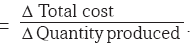
This concept is used in various ways as an aid to decision making. It could be used to determine the average level of wages earned by a given group of workers, or to determine the average sales made by a team of salespersons. In Economics, the concept of the average is very important. For example, economists use the concept in analysing investment and production decisions. They will therefore talk about the average cost of production which is the total production divided by the number of units produced, as opposed to the average revenue which is the total revenue divided by the number of units sold. Comparison of the two averages can indicate the direction in which a business is going.

Average is similar to arithmetic mean. It is calculated as the sum of items divided by number of items. It measures how much does a single variable contribute to a total. i.e

In Economics we are interested in variables like

a) Average costs (AC) 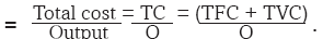This is the cost per units of output. How much expense does producing each unit of output take.

b) Average product (AP) = 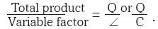 This is output per unit of the variable factor. For instance if you employ ten workers (units of labour) and all together carry 1000 bricks in an hour. How many bricks will each person have carried.

c) Average revenue (AR) =  This is revenue per unit of output sold. How much income does each unit of output produced and sold bring to the firm.

4.2.5.2 Index Numbers

Activity 4.12

Index numbers in Economics are usually used to establish changes in the cost of living of the people. They are usually constructed to show the difference in the price of a commodity from one period to another. In constructing such index numbers, we select one year which we belief to have been relatively stable, and call it the base year. We give this year an index value of 100. For example, if the price of sugar in 2010 was $1.00 while in 2014 it rose to $1.2, then the price would have risen in the period by 40%.

If we take 2010 to be the base year, then the index value for 2014 would be 140. The figure 140, which relates the two prices for the two years, is called the price relative. If this was true for a wide range of commodities, then we could assert that the cost of living has risen by 40% between 2010 and 2014.

To determine such change in the cost of living, we construct what is called a consumers cost of living index. In this case, we consider a range of commonly used consumer products and get their relative price changes in the period under review. We then get the average of this price changes so as to determine an overall change in the cost of living.

In Economics, index numbers are used in prices of commodities to arrive at simple price index, especially to determine the consumer price index.
They are also used to determine the rate of human development to derive human development index.

4.2.6 Absolute values
In making calculations, it is usual to come up with a figure that has either a plus or a minus sign. However, such a sign may not be of any importance for making the desired decision. What may be important is the magnitude of the number without any consideration of the sign. We would therefore ignore the sign. This is the idea behind the concept of absolute numbers. The absolute number is the actual number without any consideration of the sign. Thus if we have the absolute number would be 3. Same case for a sign.

In Economics, when we talk about elasticity of demand, the coefficient of elasticity could be either positive or negative. However, for decision-making purposes, it is the absolute number that is considered.

Unit Summary
In this unit, the following were covered:
• Linear equations and graphs
• Non-linear equations and graphs
• Simultaneous equations
• Differential equations and graphs
• Rations, proportions and percentages
• Reciprocals
• Averages and index numbers
• Absolute values

Unit Assessment 4

Every year, our country prepares an annual budget. The allocations for every sector are always in percentages or some estimated amount.
Using the last annual budget,
(a) Represent the information on a graph.(b) Suggest reasons why some sectors get a higher share of the budget than others.