Topic outline
UNIT1: COMPLEX NUMBERS
Key unit competence
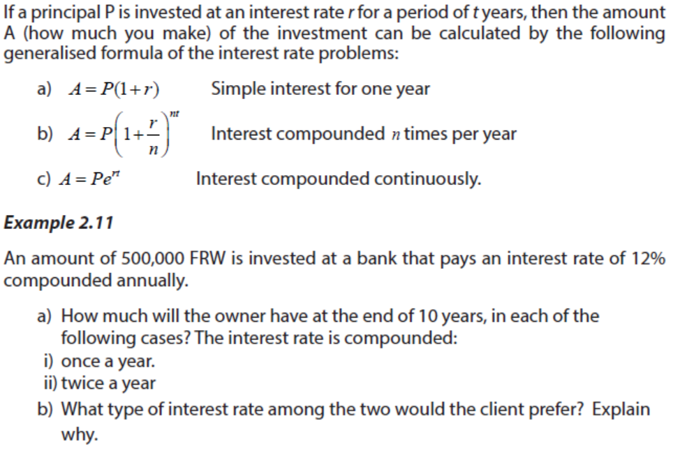
Perform operations on complex numbers in different forms and use them to solverelated problems in Physics, Engeneering, etc.
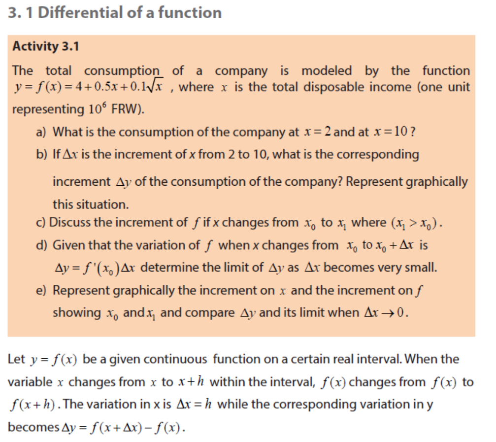
Introductory activity
Consider the extension of sets of numbers previously learnt from natural numbers
to real numbers. It is actually very common for equations to be unsolved in one
set of numbers but solved in another.
Let us find the solution of the following quadratic equations in the set of realnumbers:
1. 1 Algebraic form of Complex numbers and their geometric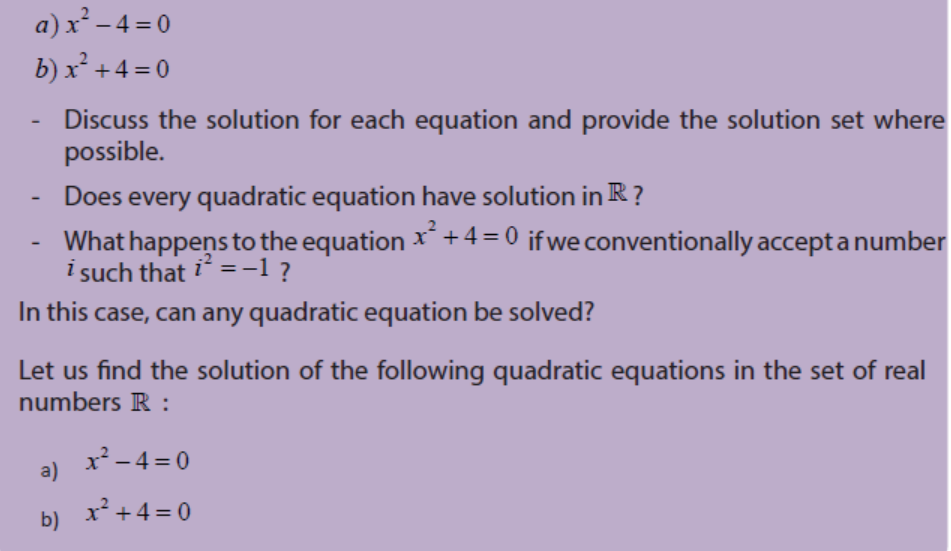
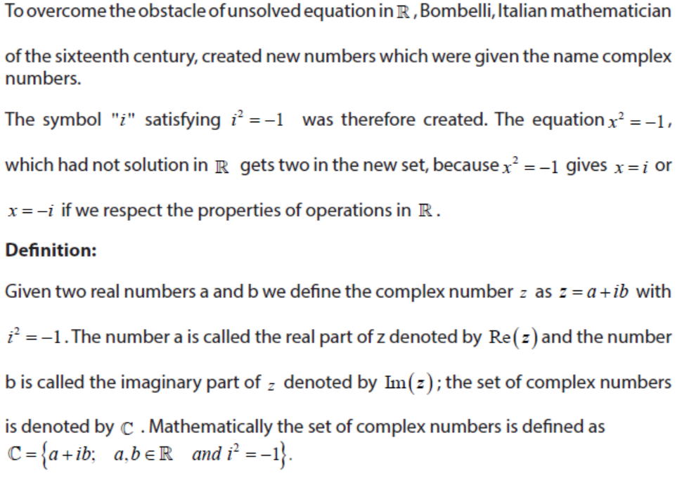
representation1.1.1 Definition of complex number
Solution
Each of these numbers can be put in the form a + ib where a and b are real numbersas detailed in the following table:
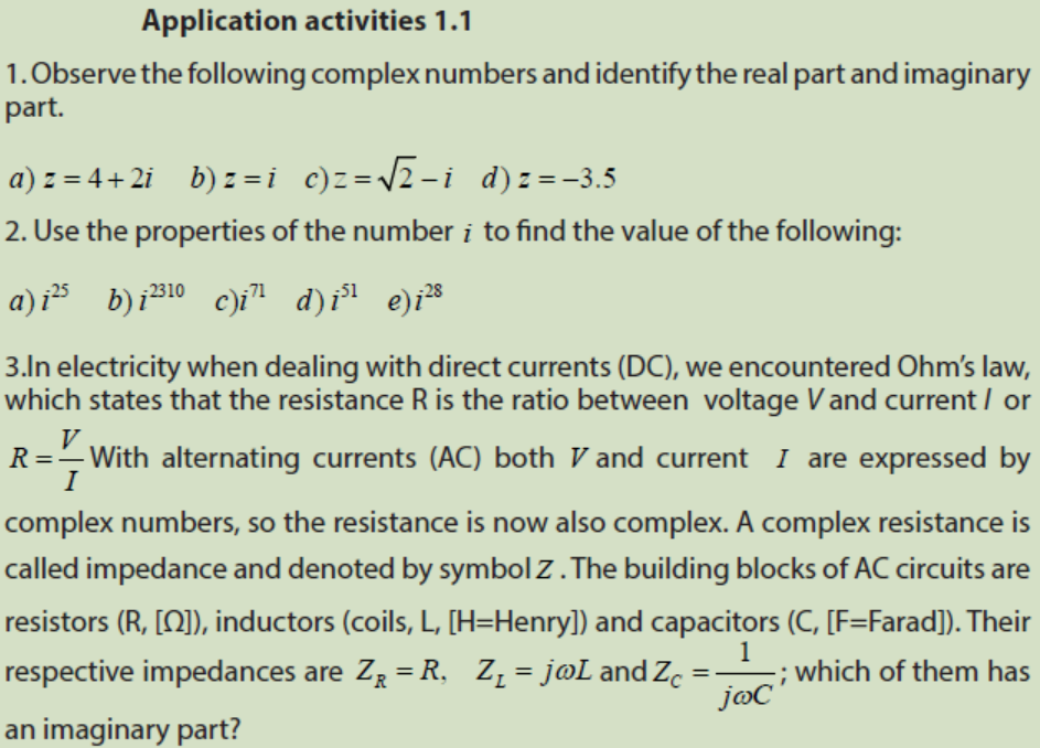
Complex numbers are commonly used in electrical engineering, as well as in physics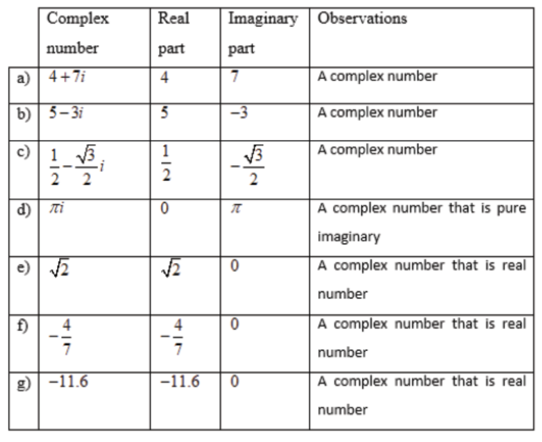
as it is developed in the last topic of this unit. To avoid the confusion between i
representing the current and i for the imaginary unit, physicists prefer to use j torepresent the imaginary unit.
As an example , the Figure 1.1 below shows a simple current divider made up of acapacitor and a resistor. Using the formula, the current in the resistor is given by
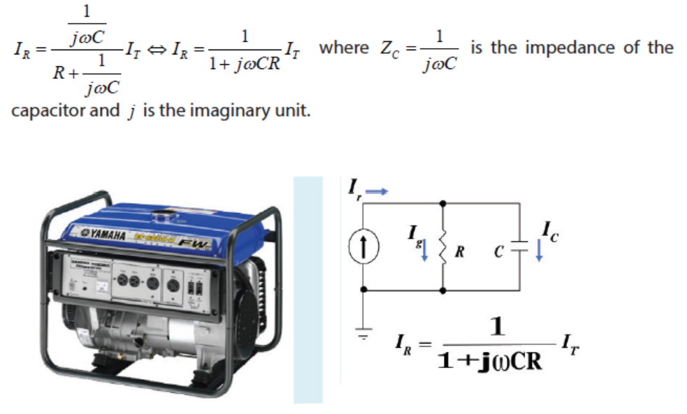
Figure 1. 1 A generator and the R-C current divider
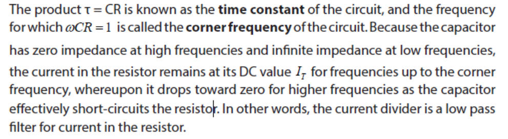
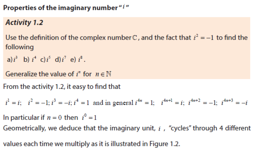
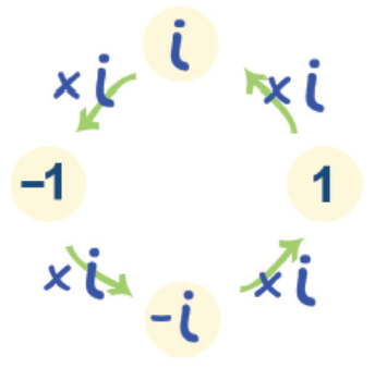
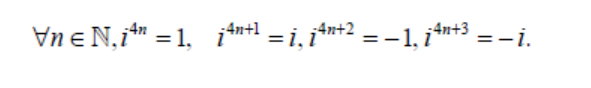
Figure 1. 2 Cycles of imaginary unit
From the figure 1.2, the following relations may be used:
1.1.2 Geometric representation of a complex number
The complex plane consists of two number lines that intersect in a right angle at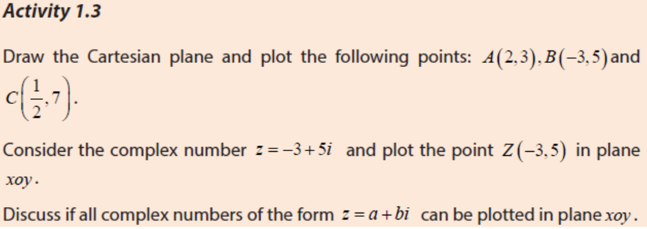
the point (0,0) . The horizontal number line (known as x − axis in Cartesian plane) isthe real axis while the vertical number line (the y − axis in Cartesian plane) is the
imaginary axis.
Every complex number z = a + bi can be represented by a point Z (a,b) in thecomplex plane.
The complex plane is also known as the Argand diagram. The new notation Z (a,b)
of the complex number z = a + bi is the geometric form of z and the point Z (a,b)is called the affix of z = a + bi . In the Cartesian plane, (a,b)is the coordinate of the

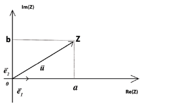
Figure 1. 3 The complex plane containing the complex number z = a + bi
Complex impedances in series
In electrical engineering, the treatment of resistors, capacitors, and inductors can
be unified by introducing imaginary, frequency-dependent resistances for the latter
two (capacitor and inductor) and combining all three in a single complex number
called the impedance. If you work much with engineers, or if you plan to become
one, you’ll get familiar with the RC (Resistor-Capacitor) plane, just as you will with
the RL (Resistor-Inductor) plane.
Each component (resistor, an inductor or a capacitor) has an impedance that can be
represented as a vector in the RX plane. The vectors for resistors are constantregardless of the frequency.
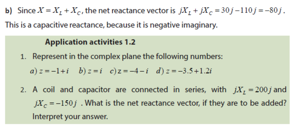
together when coils and capacitors are in series. Thus , X = XL + XC .
In the RX plane, their vectors add, but because these vectors point in exactly
opposite directions inductive reactance upwards and capacitive reactance
downwards, the resultant sum vector will also inevitably point either straight up ordown (Fig. 1.4).
Figure 1. 4 Pure inductance and pure capacitance represented by reactance vectors that point straight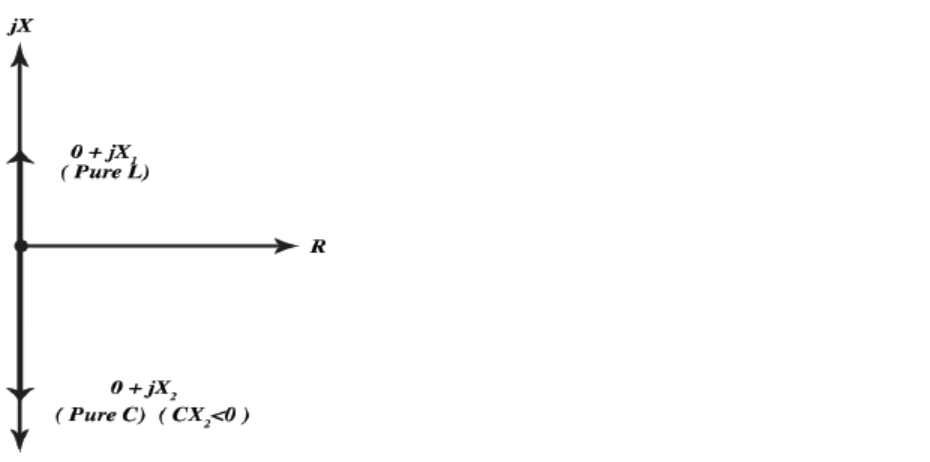
up and down.Example 1.2
Solution
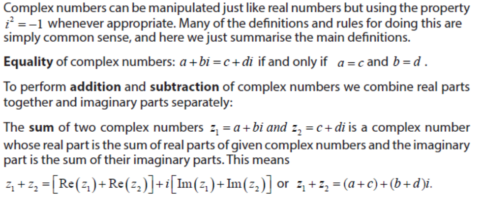
1.1.3 Operation on complex numbers
1.1.3.1 Addition and subtraction in the set of complex numbers
Adding impedance vectors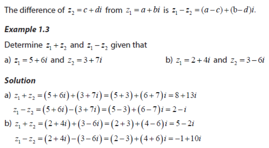
If you plan to become an engineer, you will need to practice adding and subtracting
complex numbers. But it is not difficult once you get used to it by doing a few sample
problems. In an alternating current series circuit containing a coil and capacitor,
there is resistance, as well as reactance.
Whenever the resistance in a series circuit is significant, the impedance vectors
no longer point straight up and straight down. Instead, they run off towards the
“northeast” (for the inductive part of the circuit) and “southeast” (for the capacitivepart). This is illustrated in Figure 1.5.
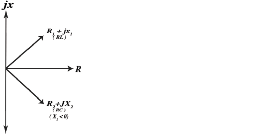
Figure 1. 5 Resistance with reactance and impedance vectors pointing “northeast “or “southeast.”
When vectors don’t lie along a single line, you need to use vector addition to be
sure that you get the correct resultant. In Figure 1.6, the geometry of vector additionis shown by constructing a parallelogram, using the two vectors Z1 = R1 + jX1 and
Z2=R2+jX2 as two of the sides. Then, the diagonal is the resultant
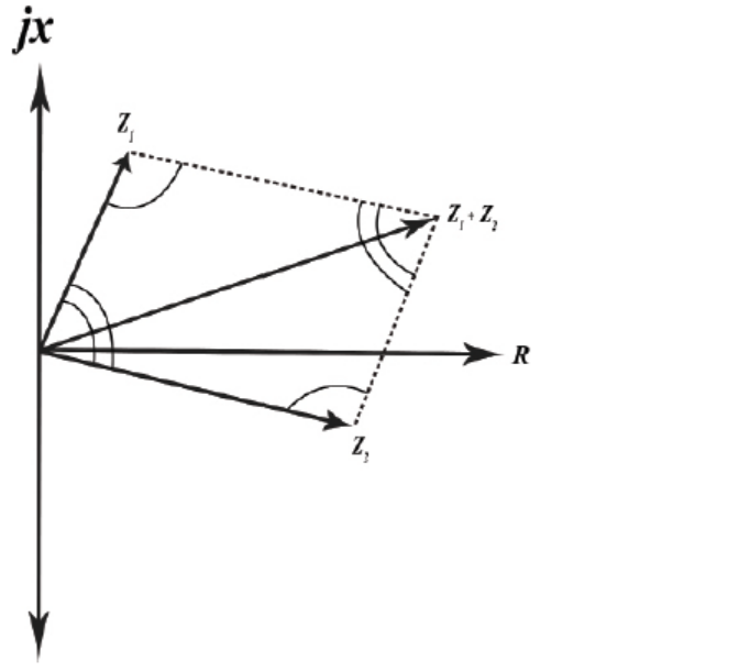
Figure 1. 6 Vector addition of impedances Z1 = R1 + jX1 and Z2 = R2 + jX2
Formula for complex impedances in series RLC circuits
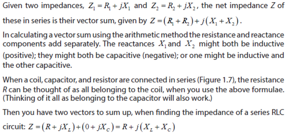
Figure 1. 7 A series RLC circuit
Example 1.4
A resistor, coil, and capacitor are connected in series with , R = 45Ω XL= 22Ω andXC = − 30Ω. What is the net impedance, Z ?
SolutionConsider the resistor to be part of the coil (inductor), obtaining two complex vectors,
45 + 22 j and0 − 30 j. Adding these gives the resistance component of
(45 + 0)Ω = 45Ω, and the reactive component of (22 j − 30 j)Ω = −8 jΩ. Therefore
the net impedance is Z = (45 −8 j)Ω .
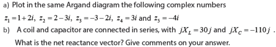
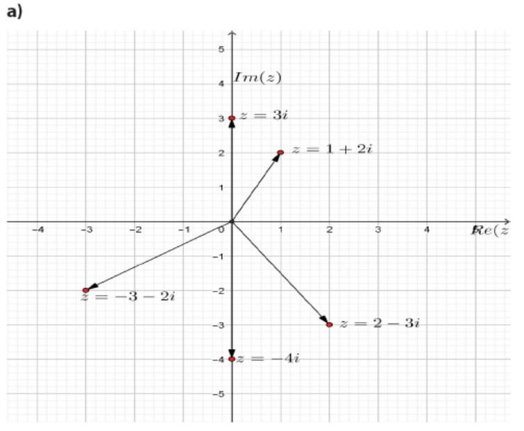
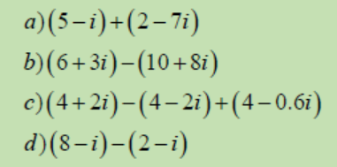
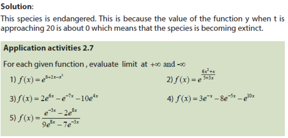
Application activities 1.3
Represent graphically the following complex numbers, and then deduce the
numerical answers from the diagrams.
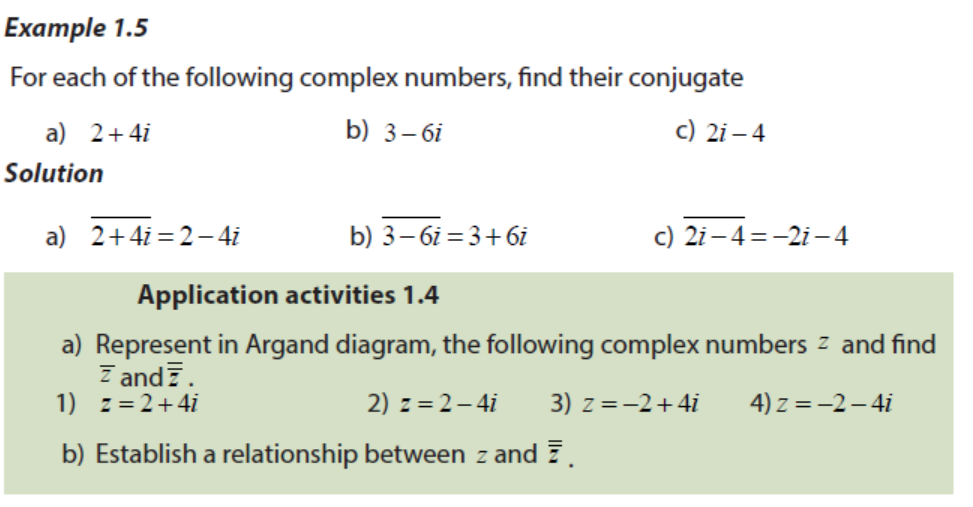
1.1.3.2 Conjugate of a complex number
Activity 1.5
In the complex plane,
1. Plot the affix of complex number z = 2 + 5i
2. Find the image P'of the point P affix of z by the reflection across the real
axis. What is the coordinate of P' ?
3. Write the complex number z ' associated to P' and discuss the relationship
between z and z ' of P' ?
4. Write algebraically the complex number z ' associated to P' and discuss therelationship between z and z '
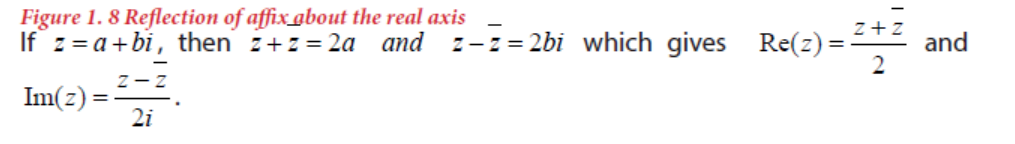
Every complex number z a bi = + has a corresponding complex number z − called
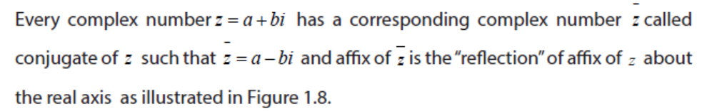
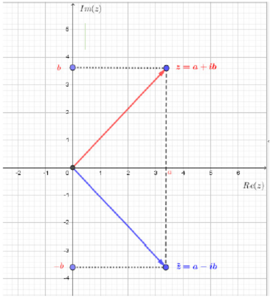
Figure 1. 8 Reflection of affix about the real axis
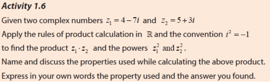
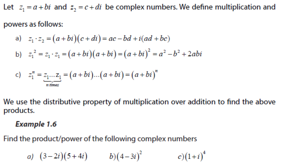
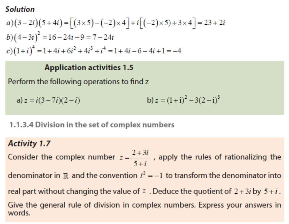
1.1.3.3 Multiplication and powers of complex number
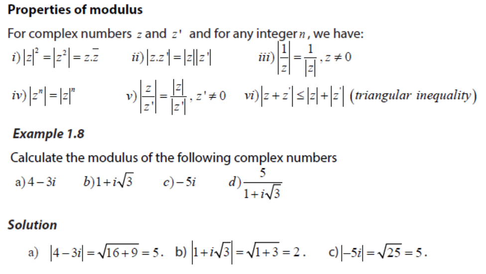
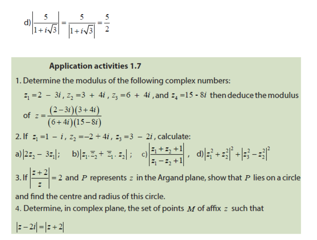
1.1.4 Modulus of a complex number
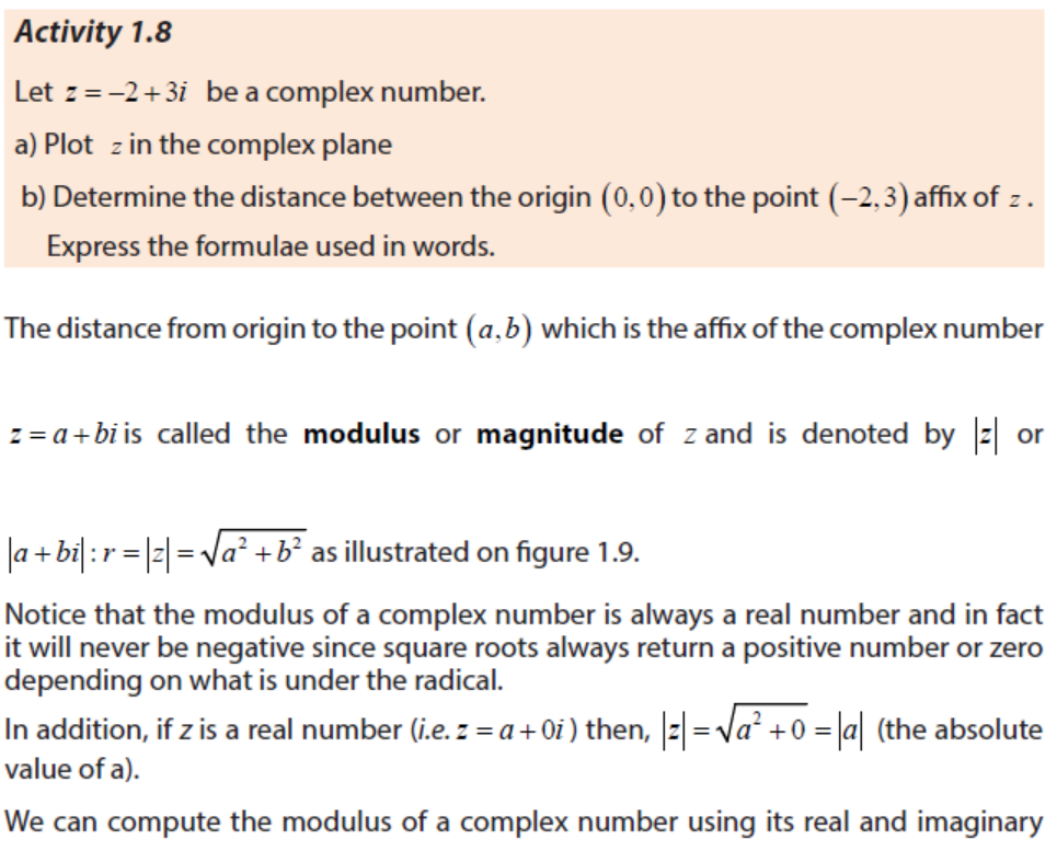

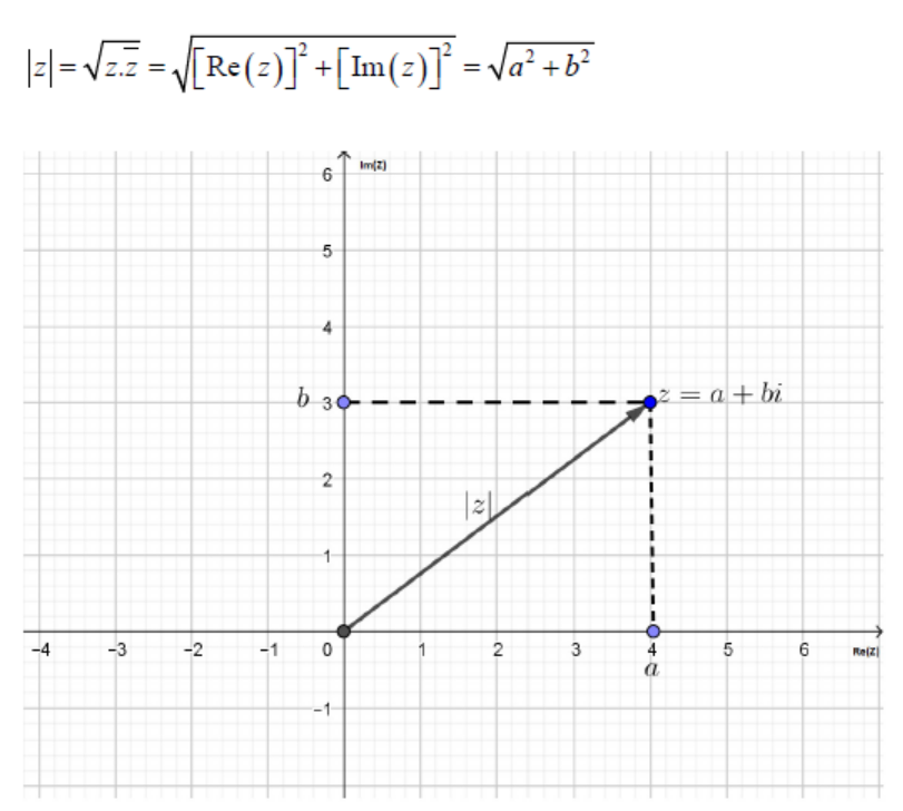
Figure 1. 9 Modulus of z = a + bi
Activity 1.11
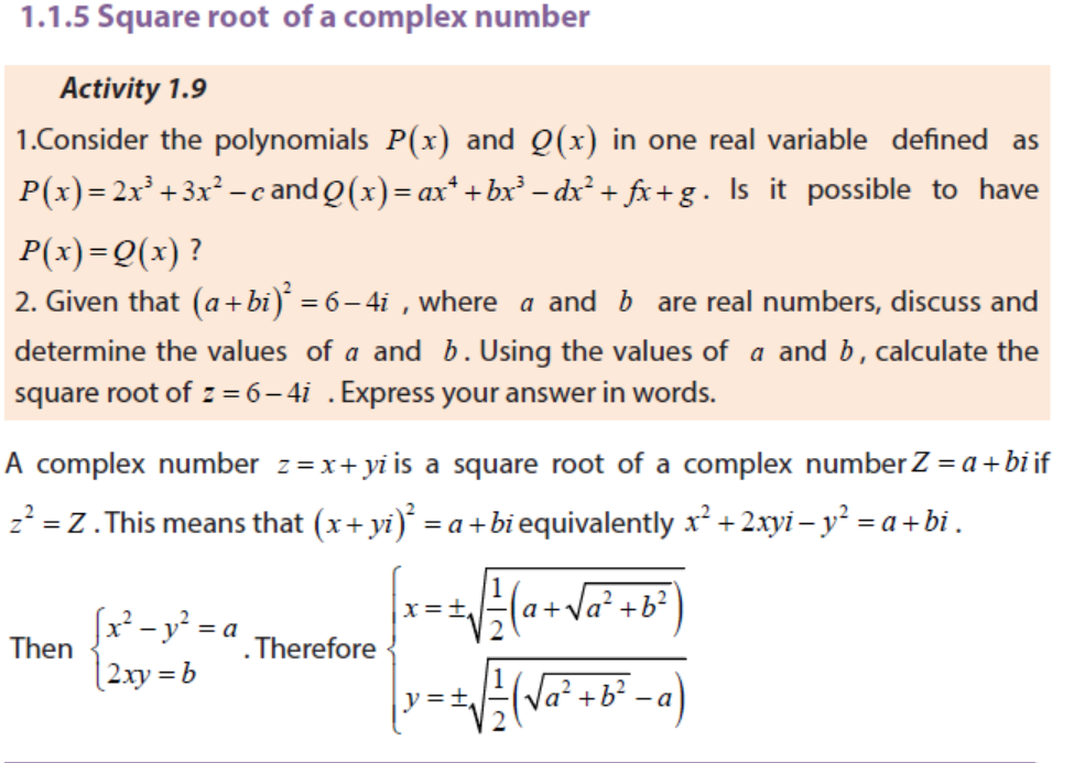
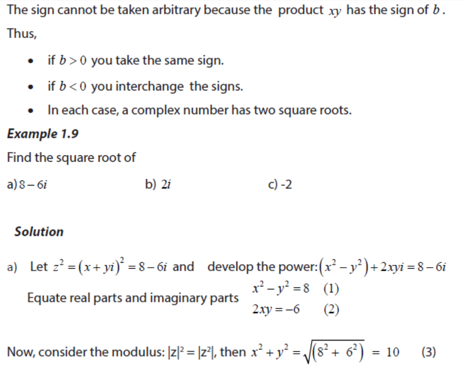
Given the quadratic equation z2 − (1+ i) = 0 , you can write it as z2 =1+ i . Calculate
the square root of 1+ i to get the value of z and discuss how to solve equations of
the form Az2 +C = 0 where A and C are complex numbers and A is differentfrom zero. Express in words the formula used.
Solving simple quadratic equations in the set of complex numbers recalls theprocedure of how to solve the quadratic equations in the set of real numbers
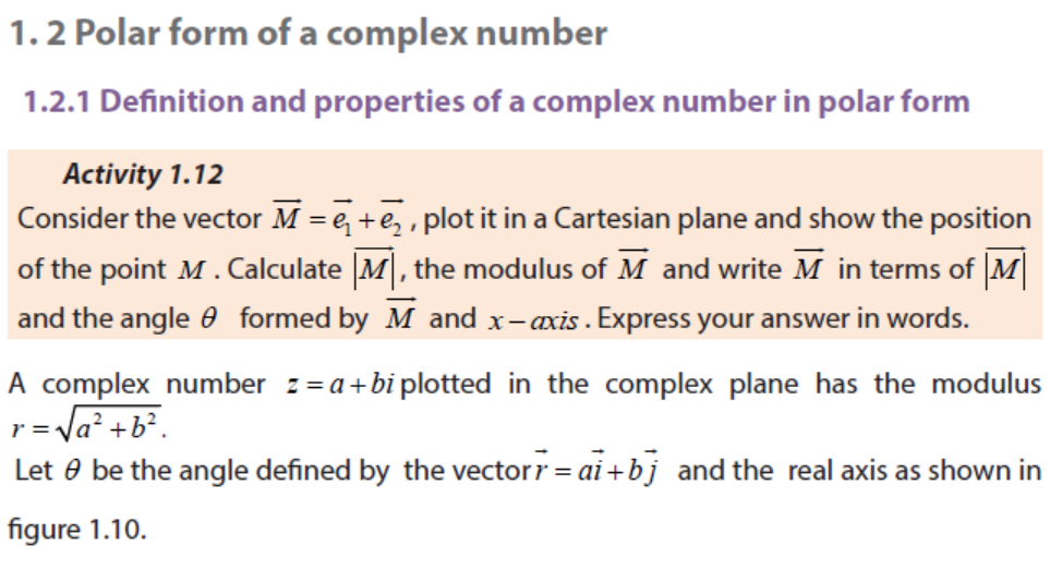
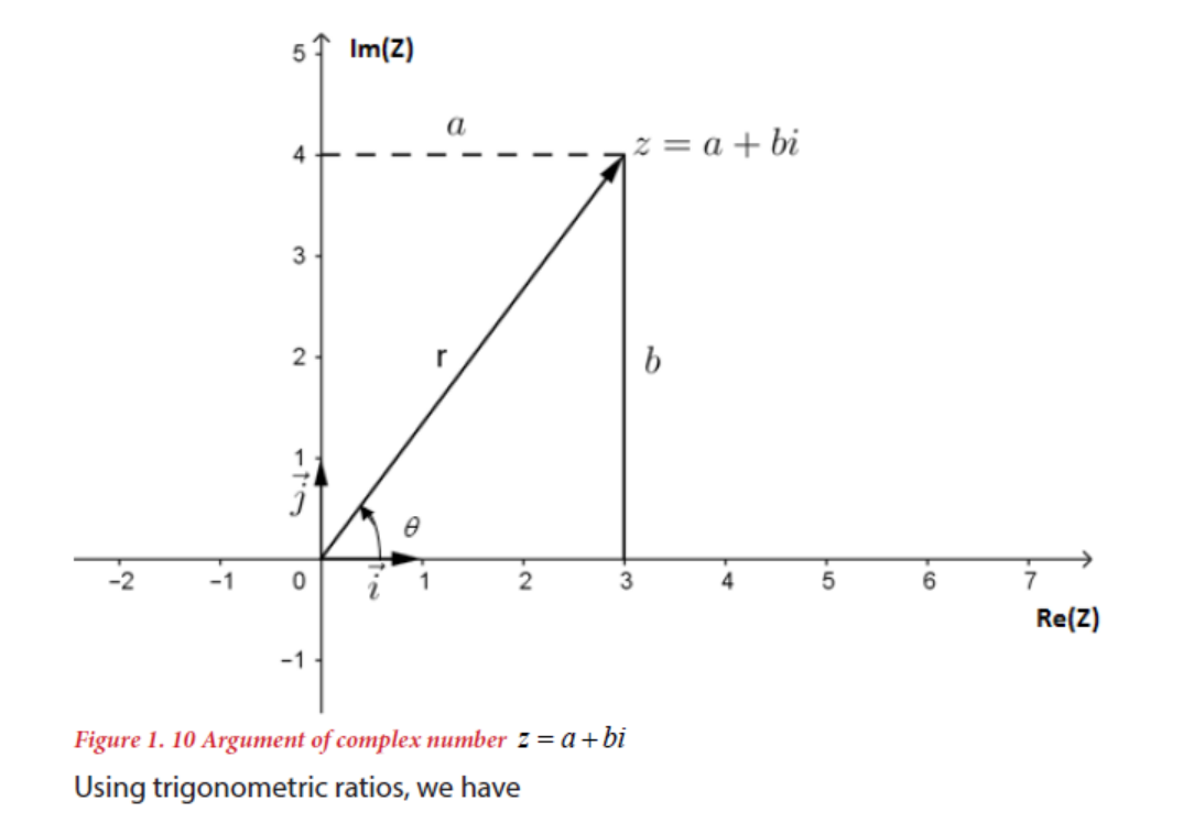
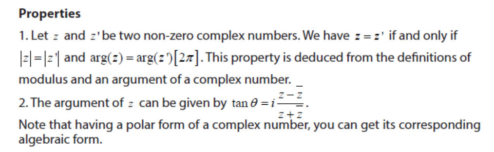
From affix of a complex number z = a + bi , there is a connection between its
modulus and angle between the corresponding vector and positive x − axis as
illustrated in figure 1.10. This angle is called the argument of z and denoted byarg ( z) .
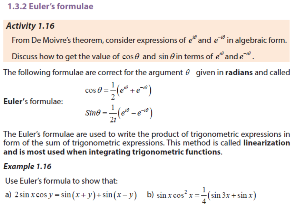
1.3 Exponential form of complex numbers
1.3.1 Definition of exponential form of a complex number
In electrical engineering, the treatment of resistors, capacitors and inductors can be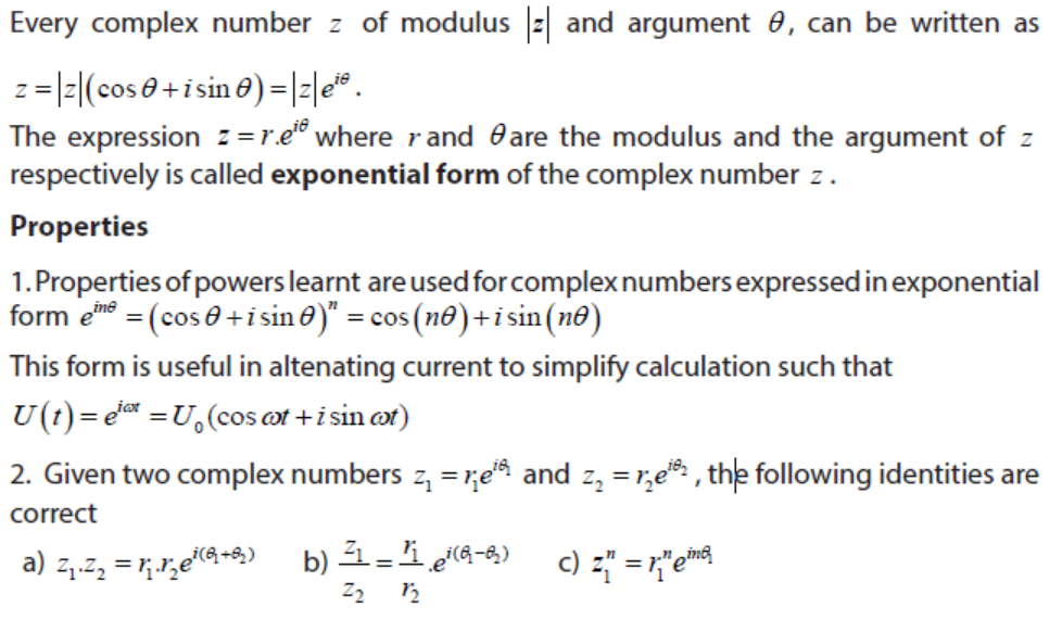
unified by introducing imaginary, frequency-dependent resistances for capacitor,
inductors and combining all three (resistors, capacitors, and inductors) in a single
complex number called the impedance. This approach is called phasor calculus. As
we have seen, the imaginary unit is denoted by j to avoid confusion with i which
is generally in use to denote electric current. Since the voltage in an AC circuit isoscillating, it can be represented as
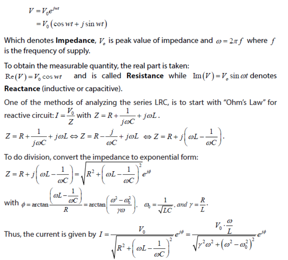
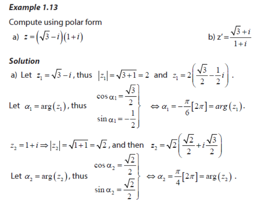
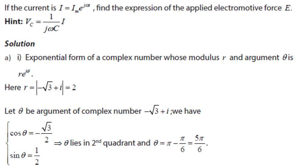
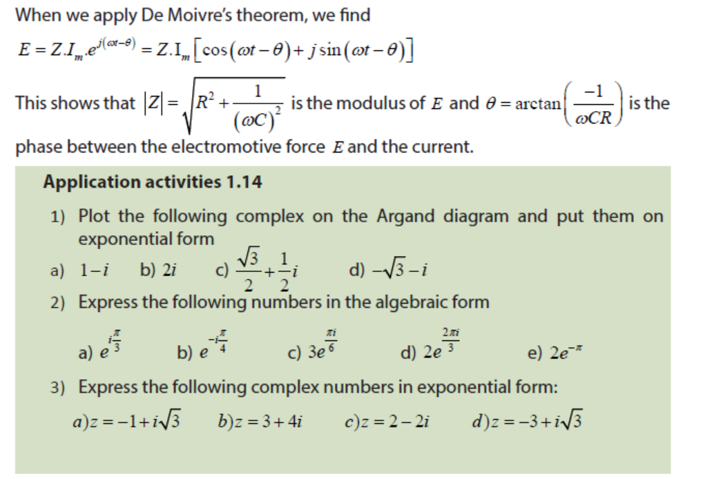
Example 1.15
a) Express the complex numbers in exponential form
Given that the same current must flow in each element, the resistor and capacitor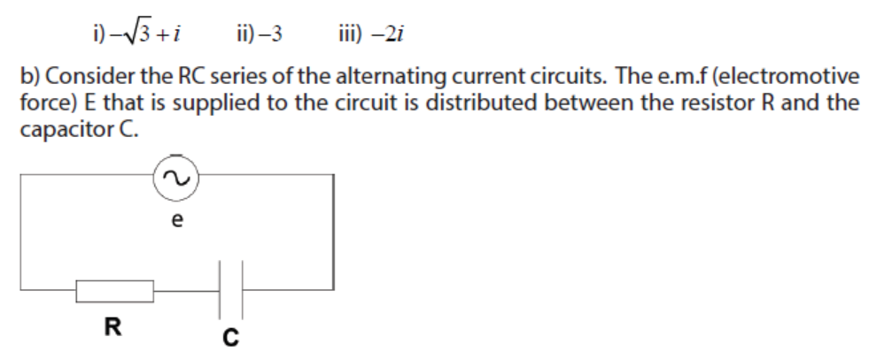
are in series such that the common current can often be taken to have the referencephase.
1.3.3 Application of complex numbers in Physics
Activity 1.17
Conduct a research from different books of the library or browse internet to
discover the application of complex numbers in other subjects such as physics,applied mathematics, engineering, etc
Complex numbers are applied in other subjects to express certain variables or
facilitate the calculation in complicated expressions. They are mostly used in electrical
engineering, electronics engineering, signal analysis, quantum mechanics, relativity,
applied mathematics, fluid dynamics, electromagnetism, civil and mechanical
engineering. Let look at an example from civil and mechanical engineering.
An alternating current is a current created by rotating a coil of wire through amagnetic field.
Figure1.11: generation of alternating current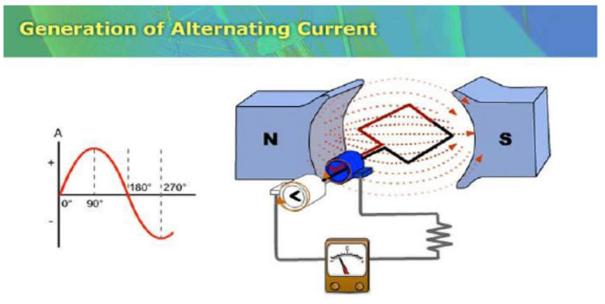
(Source: https://www.google.com/imgres?imgurl=https://image.pbs.org/poster_images)
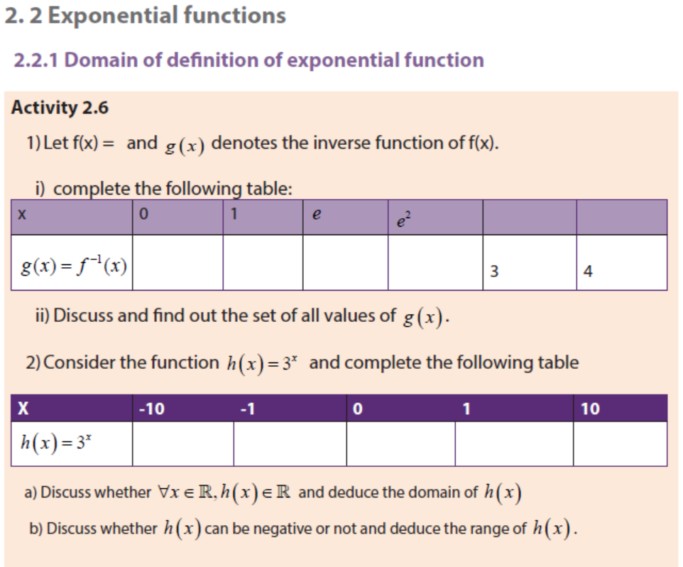
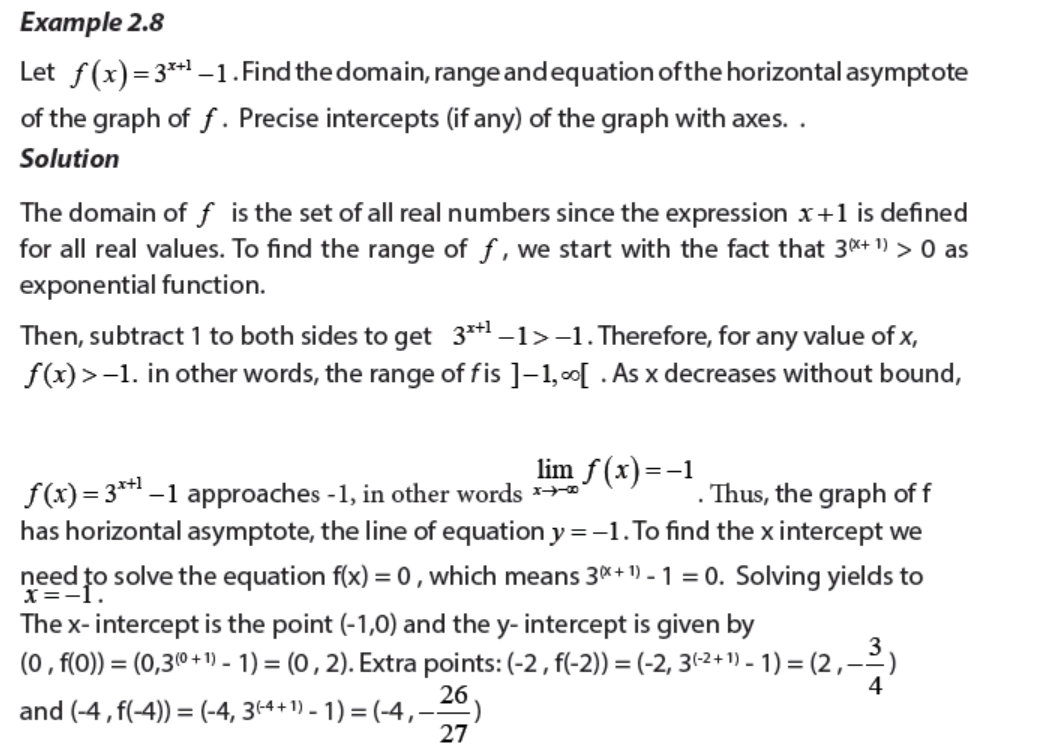
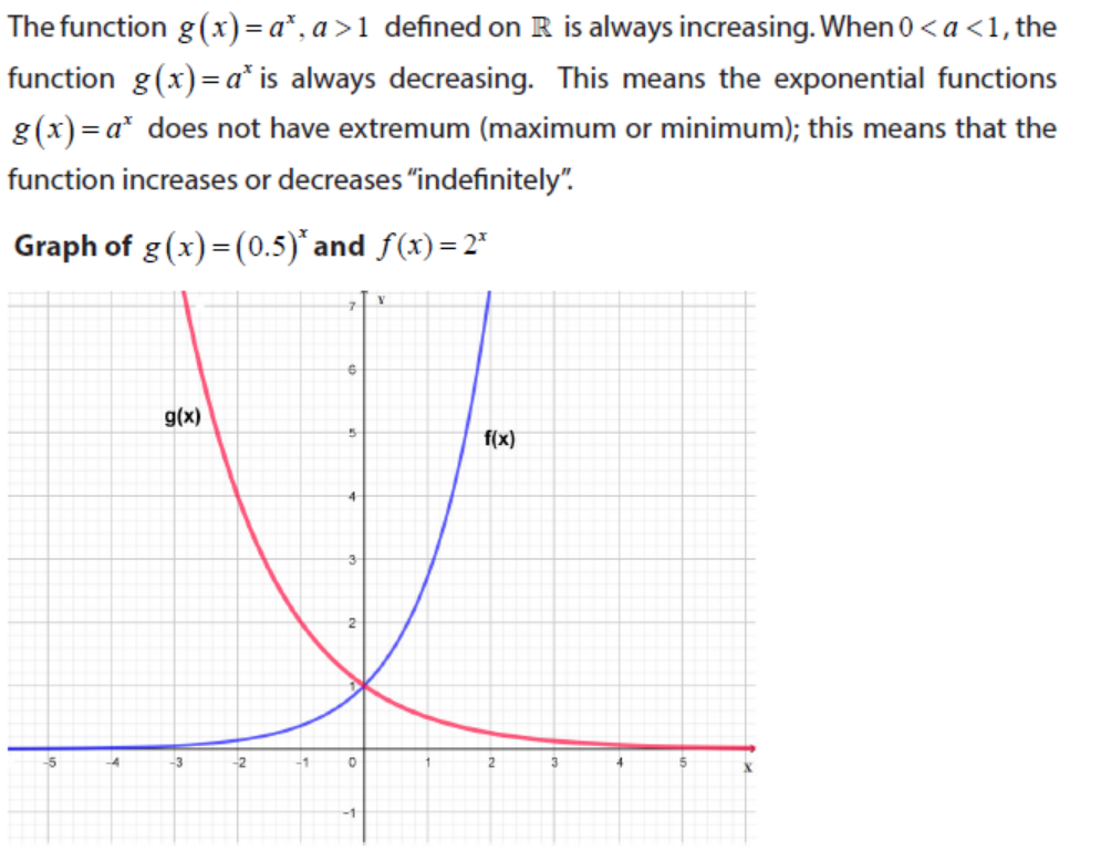
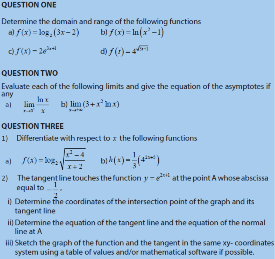
UNIT2: LOGARITHMIC AND EXPONENTIAL FUNCTIONS
UNIT2: LOGARITHMIC ANDEXPONENTIAL FUNCTIONS
UNIT2: LOGARITHMIC AND EXPONENTIAL FUNCTIONS
Key unit competence
Extend the concepts of functions to investigate fully logarithmic and exponential
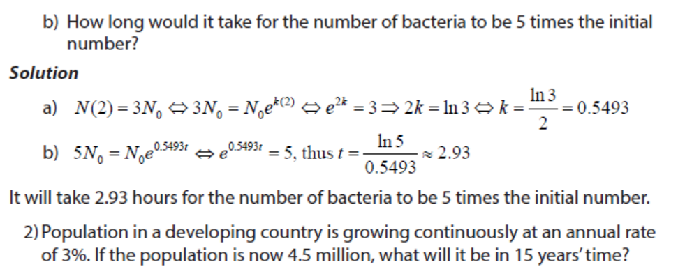
functions and use them to model and solve problems about interest rates, populationgrowth or decay, magnitude of earthquake, etc.
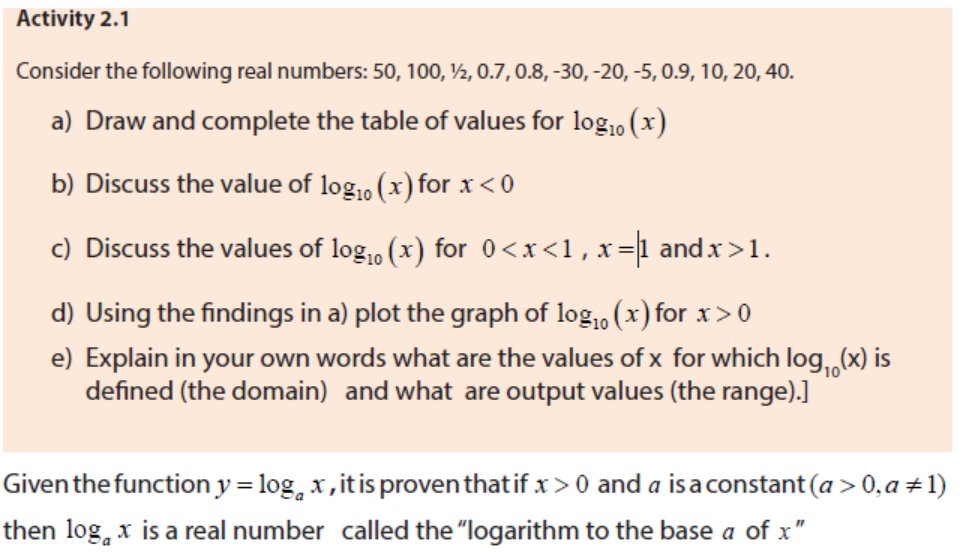
Introductory activity
The Accountant for a Health Center receives money from patients in an interesting
way so that the money he/she earns each day doubles what he/she earned the
previous day. If he/she had 200USD on the first day and by taking t as the number
of days, discuss the money he/she can have at the tth day through answering the
following questions:
a) Draw the table showing the money this Health Center Owner will have on
each day starting from the first to the 10th day.
b) Plot these data in rectangular coordinates
c) Based on the results in a), establish the formula for the Health Center
Owner to find out the money he/she can earn on the nth day. Therefore, if t
is the time in days, express the money F (t ) for the economist.
d) Now the Health Center Owner wants to possess the money F under the
same conditions, discuss how he/she can know the number of daysnecessary to get such money from the beginning of the business.
From the discussion, the function F (t ) found in c) and the function Y (F ) found in
d) are respectively exponential function and logarithmic functions that are needed
to be developed to be used without problems. In this unit, we are going to study the
behaviour and properties of such essential functions and their application in real lifesituation.
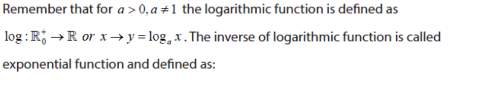
2. 1 Logarithmic functions2.1.1 Domain of definition for logarithmic function
If the base is 10, it is not necessary to write the base, and we say decimal logarithm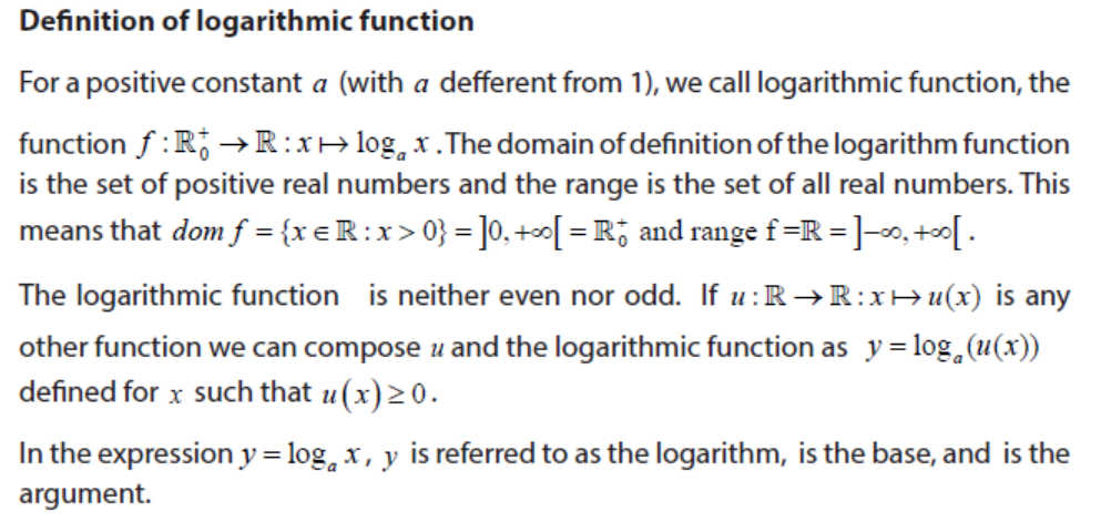
or common logarithm or Brigg’s logarithm. So, the notation will become y = log x . If
the base is e (where e =2.718281828…), we have Neperean logarithm or naturallogarithm denoted by y = ln x instead of loge y = x as we might expect.
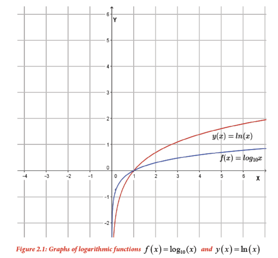
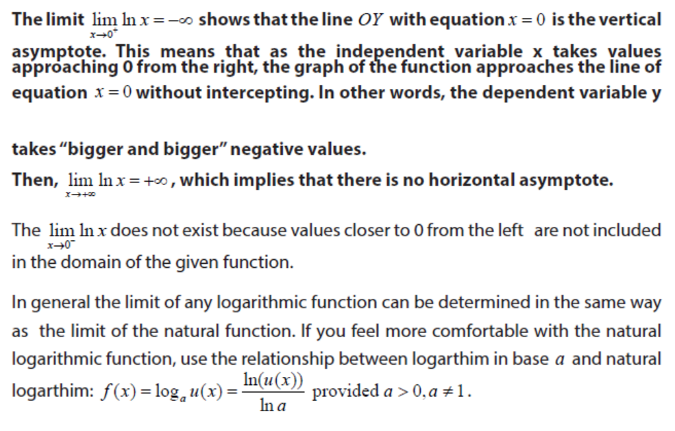
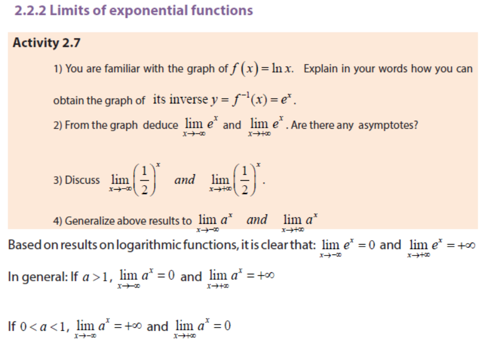
2.1.2 Limits and asymptotes of logarithmic functions
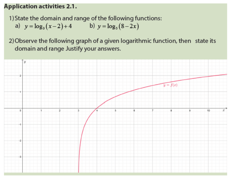
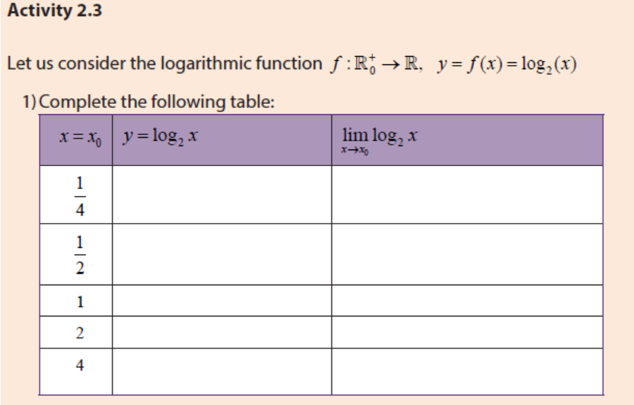
Activity 2.2
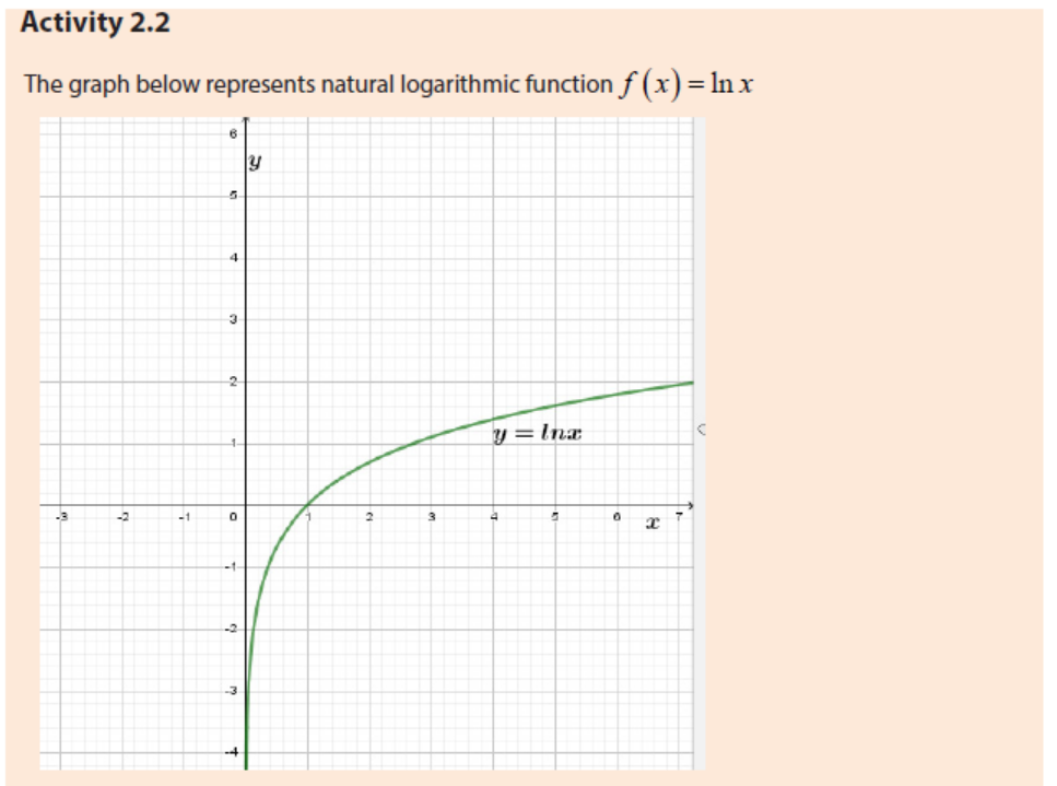
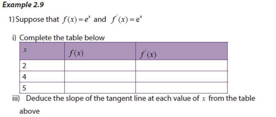
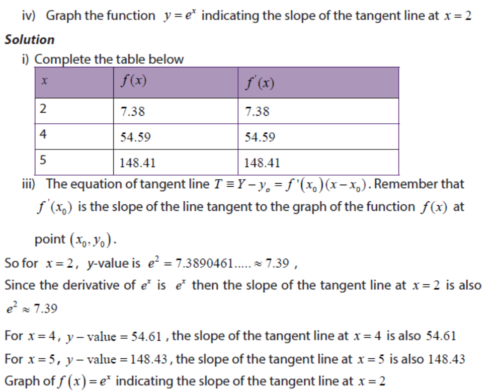
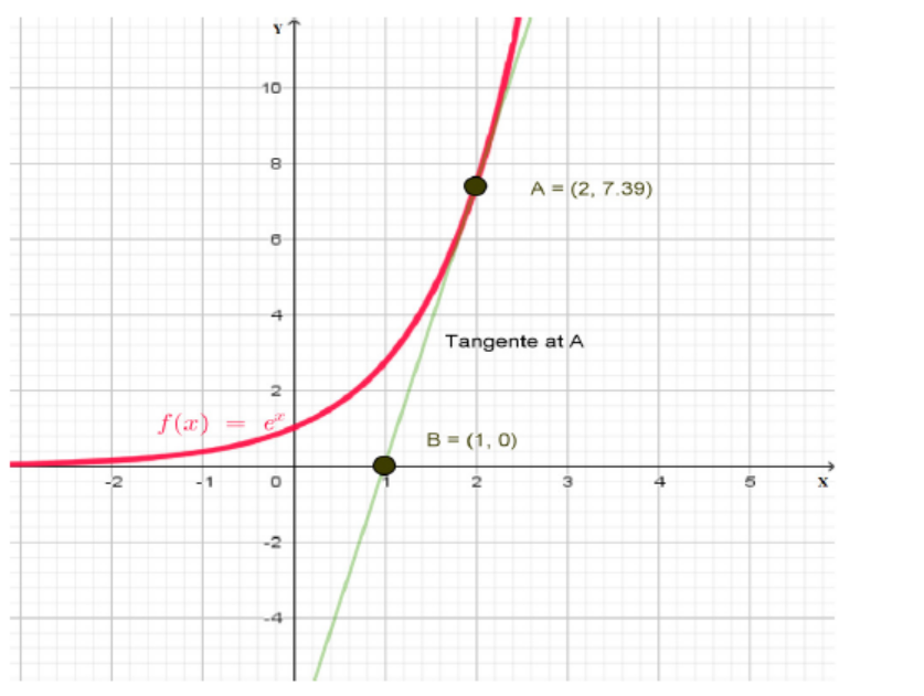
Consider the form of this graph then by using calculator, complete the table below to answer the
questions that follow.
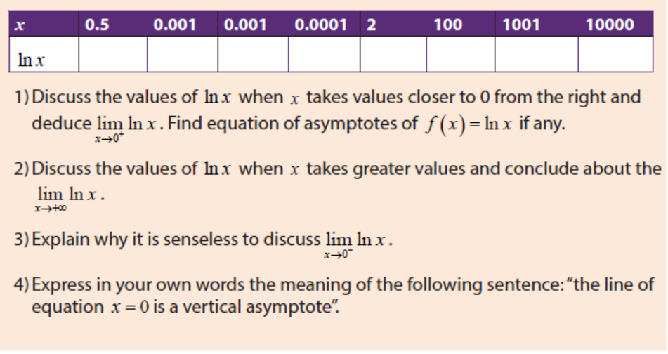
2.1.3 Continuity and asymptote of logarithmic functions
• The logarithmic function is increasing and takes its values (range) from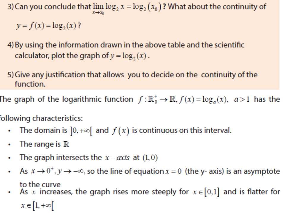
negative infinity to positive infinity.
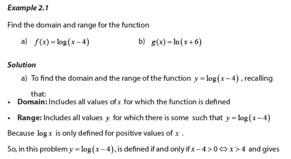
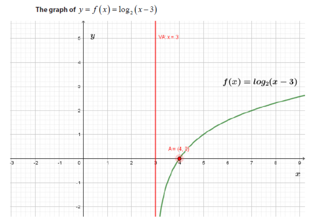
Example 2.3
Let us consider the logarithmic function y = log2 (x − 3)
a) What is the equation of the asymptote line?
b) Determine the domain and range
c) Find the x − intercept.
d) Determine other points through which the graph passes
e) Sketch the graph
Solution
a) The basic graph of 2 y = log x has been translated 3 units to the right, so the line L ≡ x = 3
is the vertical asymptote.
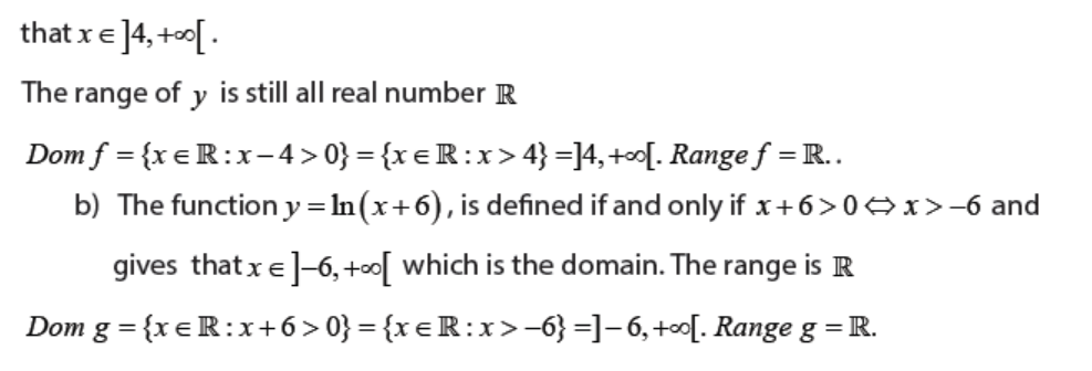
b) The function y = log2 (x − 3) is defined for x − 3 > 0
So, the domain is ]3,+∞[ .The range is
c) The intercept is (4, 0) since log2 (x − 3) = 0⇔ x = 4
d) Another point through which the graph passes can be found by allocating an arbitrary value
to x in the domain then compute y.
For example, when x = 5, y = log2 (5 − 3) = log2 2 =1 which gives the point (5,1) .
Note that the graph does not intercept y-axis because the value 0 for x does not belong tothe domain of the function.
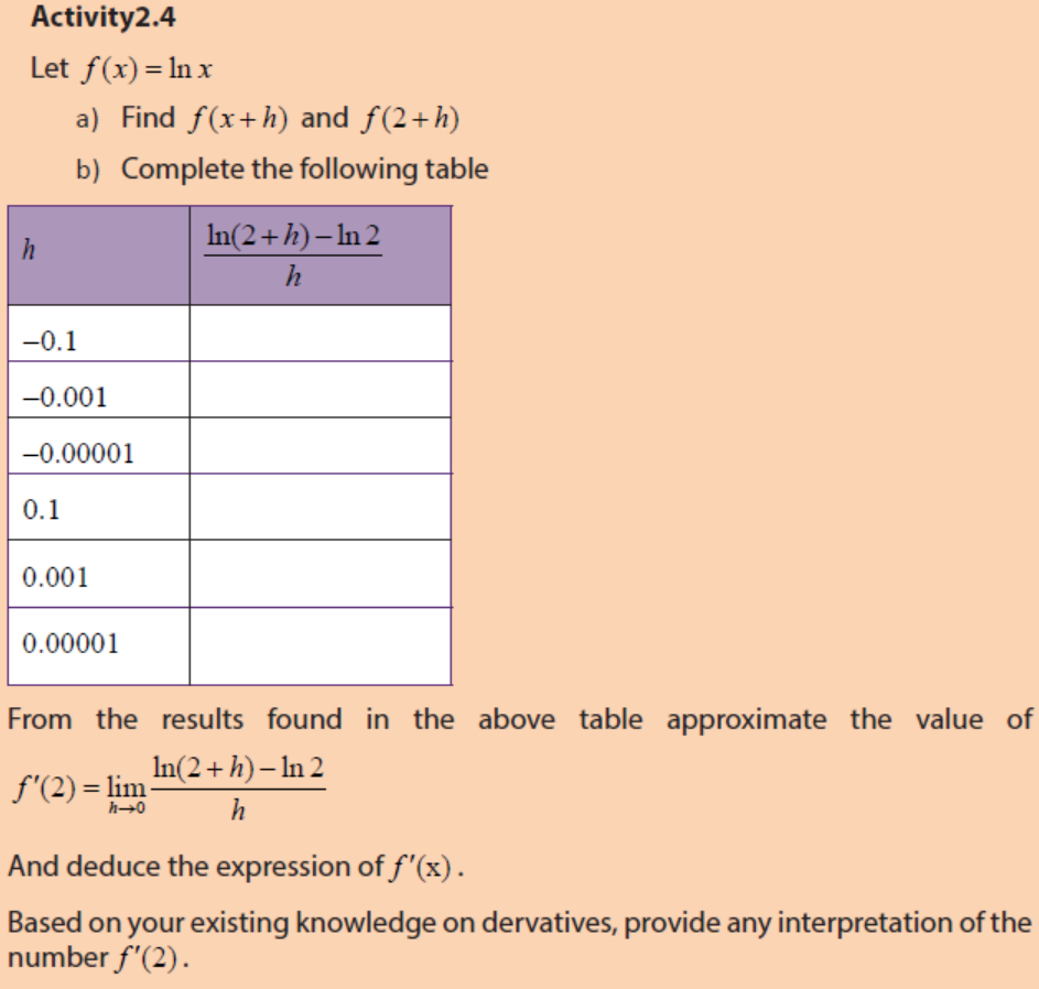
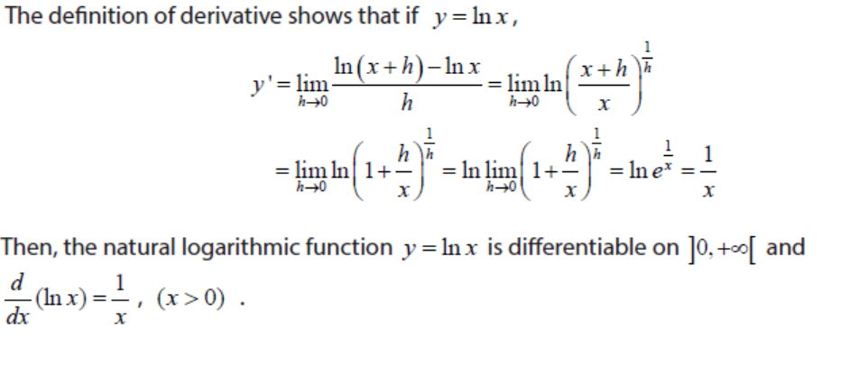
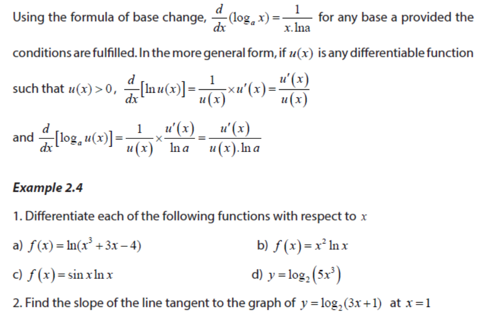
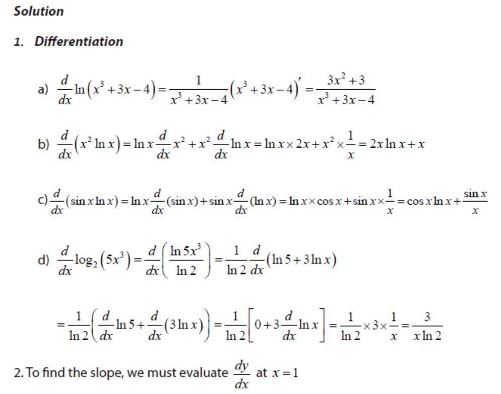
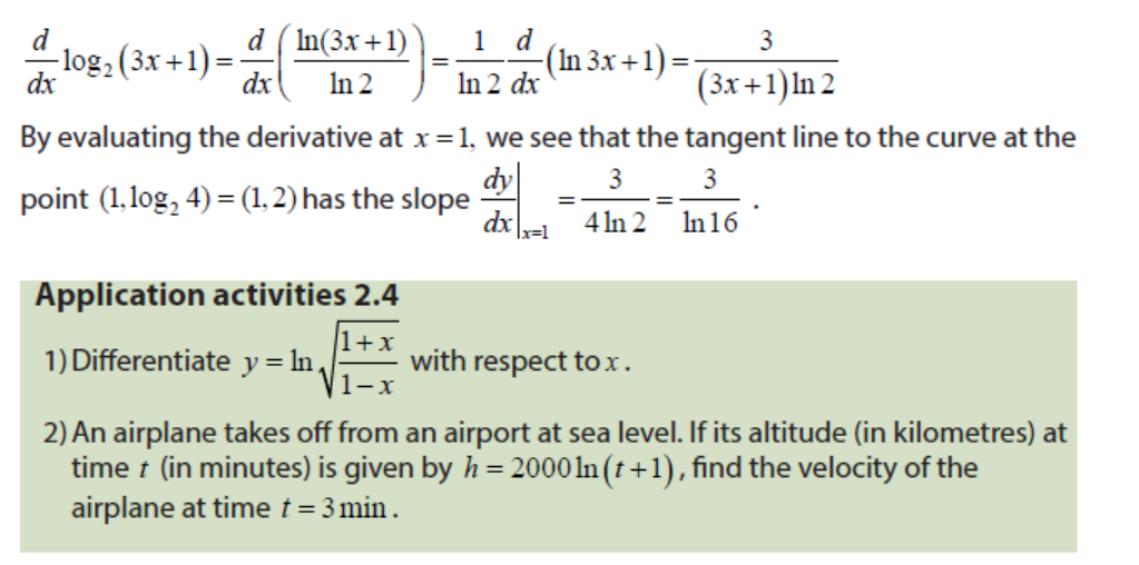
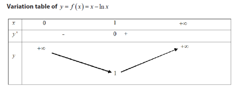
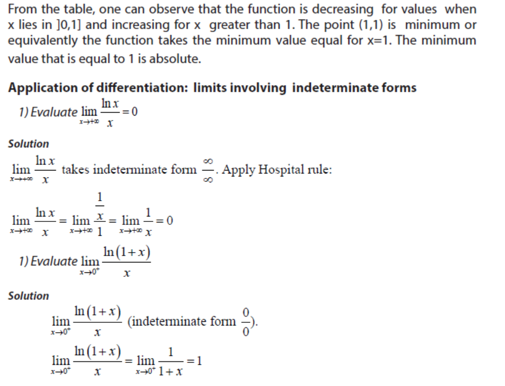
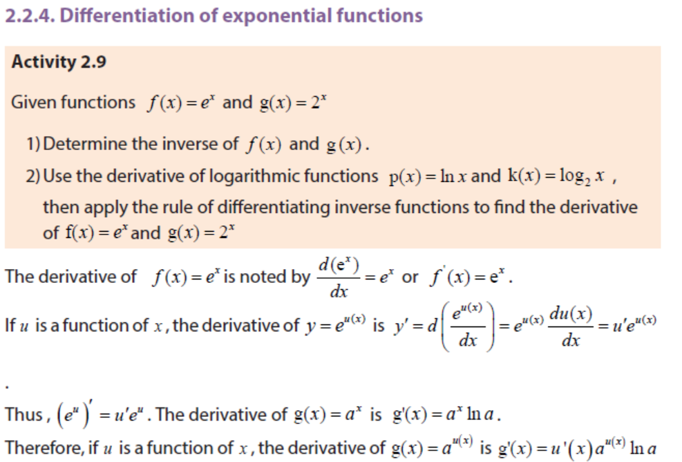
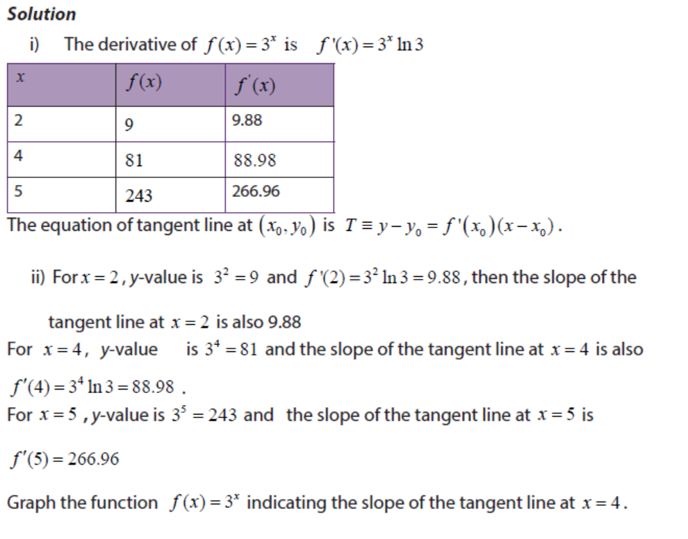
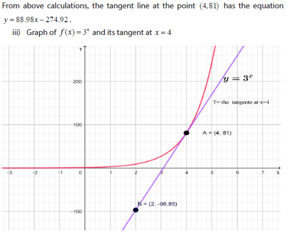
2.1.4. Differentiation of logarithmic functions
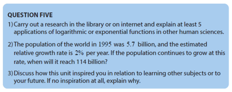
2. 3 Applications of logarithmic and exponential functions
Logarithmic and exponential functions are very essential in pure sciences, social
sciences and real life situations. They are used by bank officers to deal with interests
on loans they provide to clients. Economists and demographists use such functions
to estimate the number of population after a certain period and many researchers
use them to model certain natural phenomena. We are going to develop some ofthese applications.
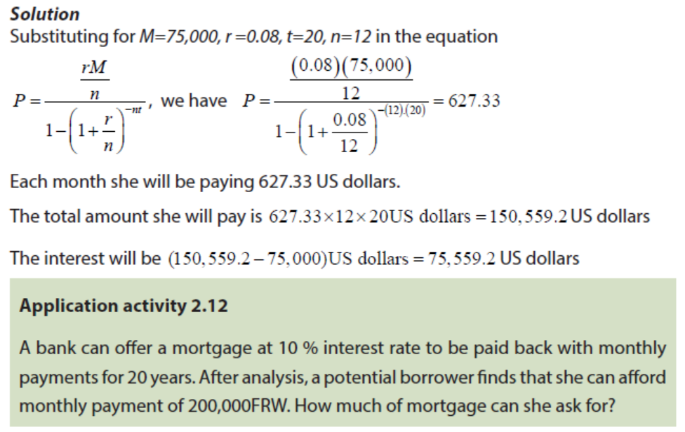
When a person gets a loan (mortgage) from the bank, the mortgage amount M, the
number of payments or the number t of years to cover the mortgage, the amount
of the payment P, how often the payment is made or the number n of payments peryear, and the interest rate r, it is proved that all the 5 components are related by
Example 2.12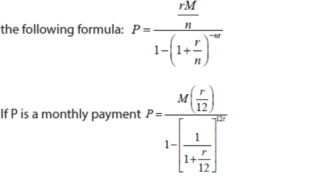
A business woman wants to apply for a mortgage of 75,000 US dollars with an
interest of 8% per month that runs for 20 years. How much interest will she pay overthe 20 years?

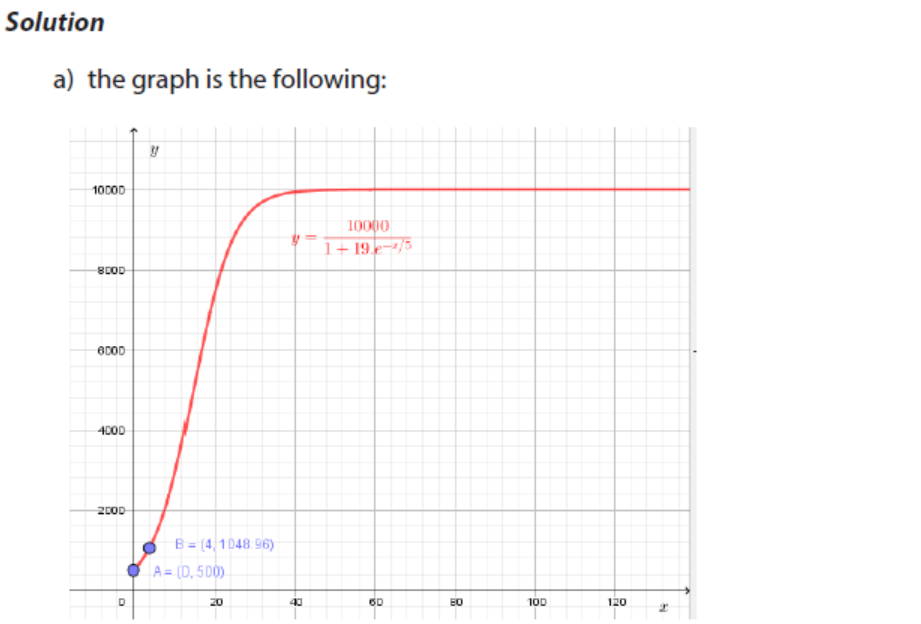
b) At the beginning, (t = 0), the number of fish is 500. After 4 months (t = 4),
the number of fish is 4,1048.
c) As the time x increases, the number of fish will be 10,000.
d) The population is increasing most rapidly after 4 months. This is becausethe increment of fish after 1 month is greater.
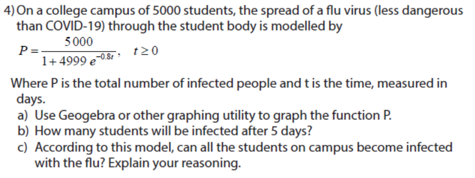
b) After 5 days, the calculator and the graph show that 54 students will be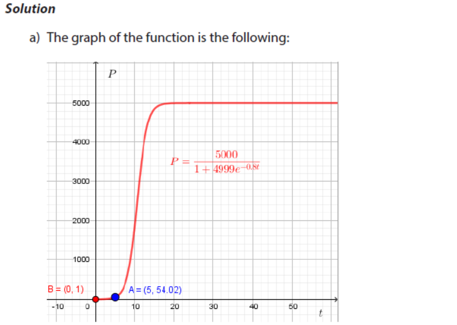
infected.
c) According to this model, when the time increases without bound, the graph
shows that all students can be infected. However, in real life, the infinite
time is not possible. Therefore, all students cannot be infected.
2.3.5 Earthquake problems
Activity 2.15
Do the research in the library or explore internet to find out how Charles Richter
tried to compare the magnitude of two earthquakes by the use of logarithmicfunction.
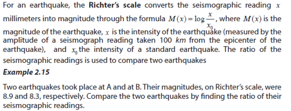
Seismographic readings are made at a distance of 100 kilometers from the epicenter
of an earthquake. If there is no earthquake, the seismographic reading is x0 = 0.001millimeter.
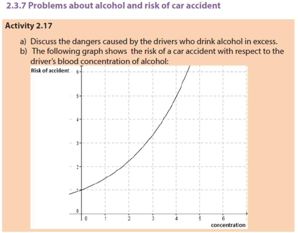
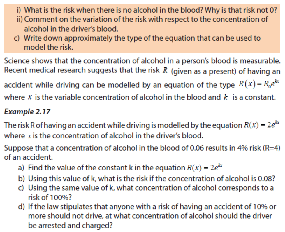
Example 2.17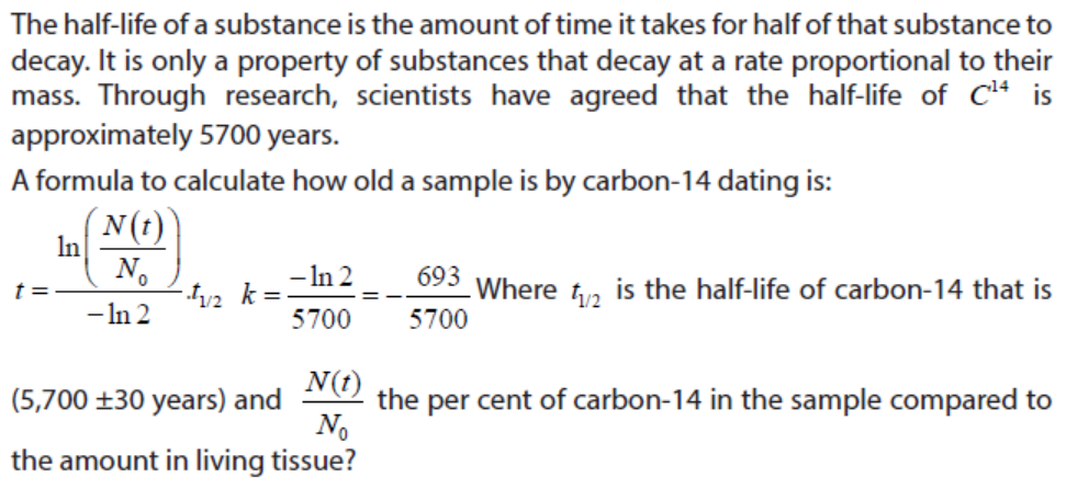
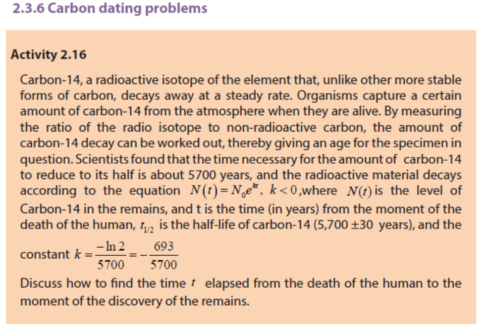
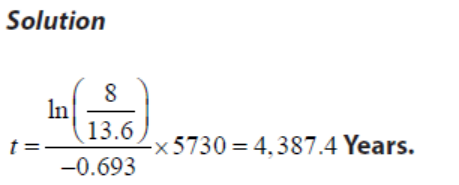
A scientist determines that a sample of petrified wood has a carbon-14 decay rate of
8.00 counts per minute per gram. What is the age of the piece of wood in years? The
decay rate of carbon-14 in fresh wood today is 13.6 counts per minute per gram, andthe half- life of carbon-14 is 5730 years.
END UNIT ASSESSMENT

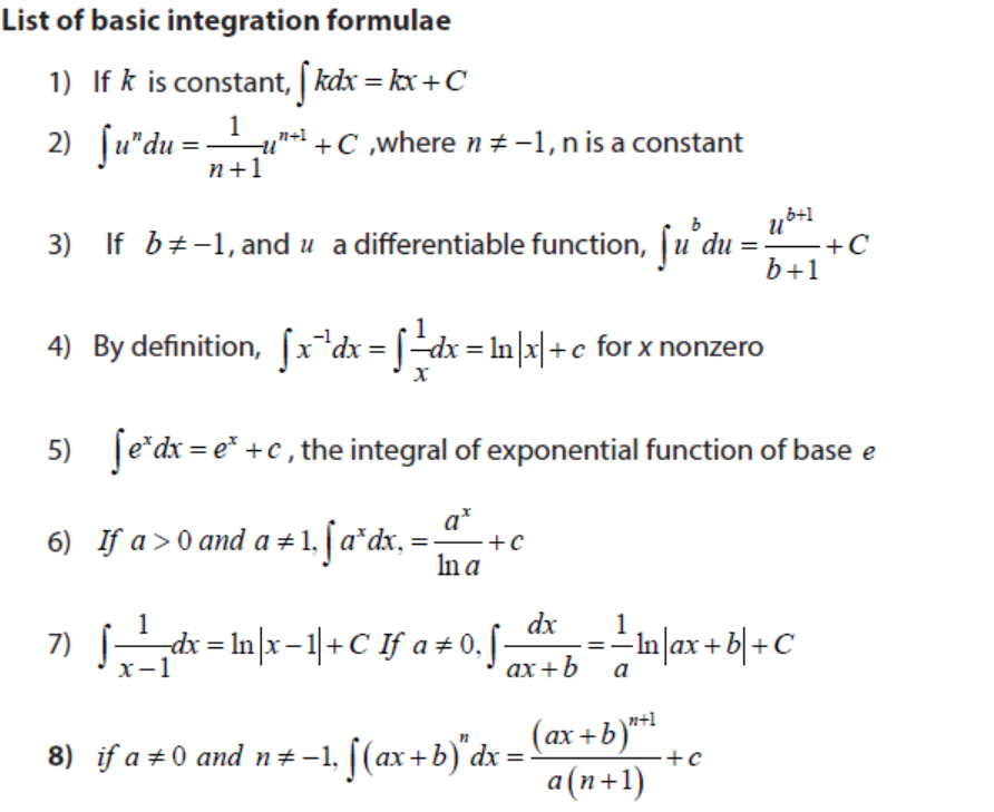
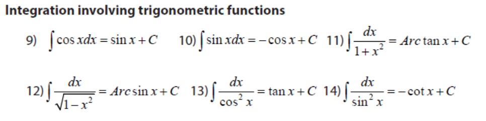
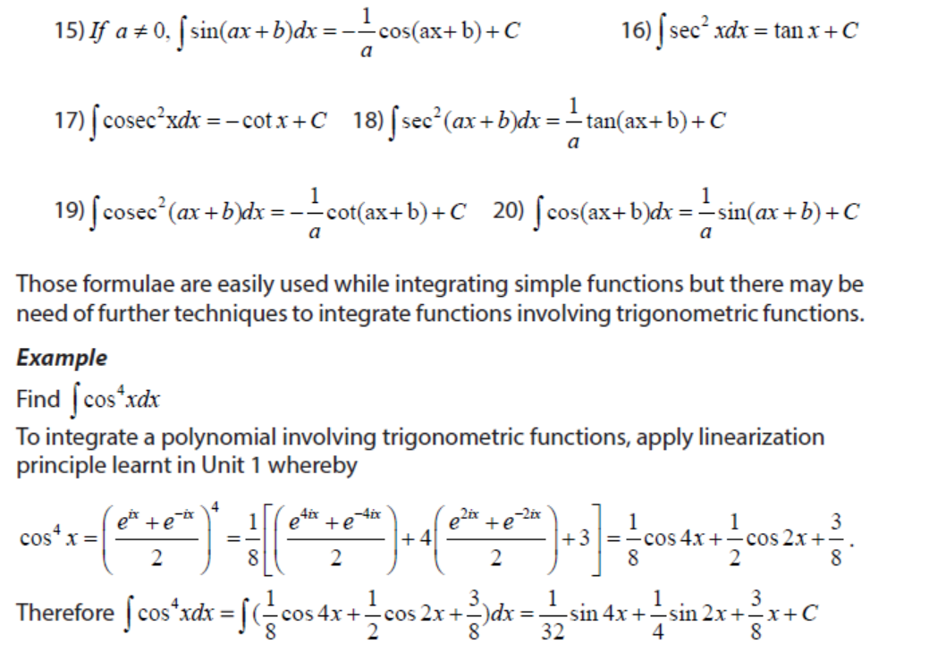
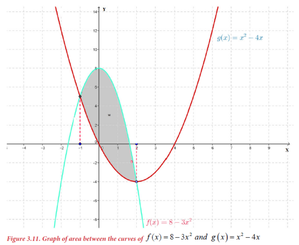
Unit 3: INTEGRATION
Unit 3: INTEGRATION
Key unit competence
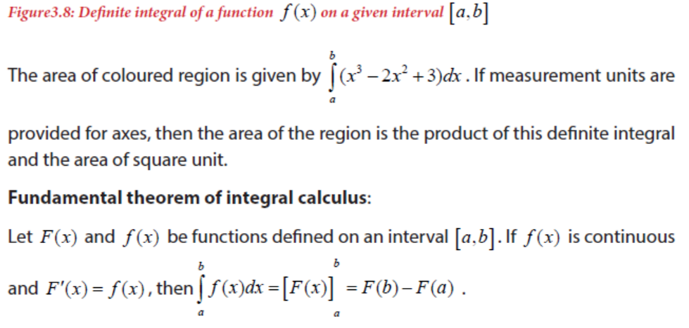
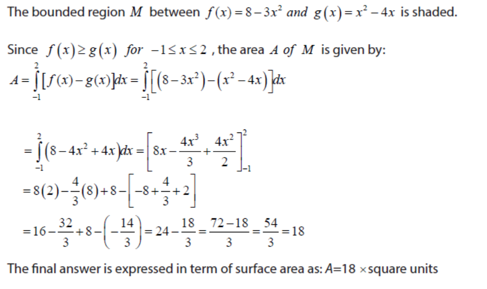
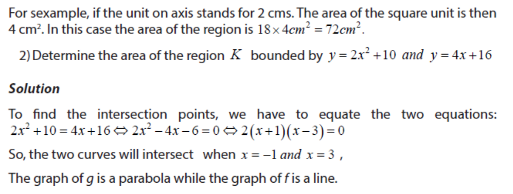
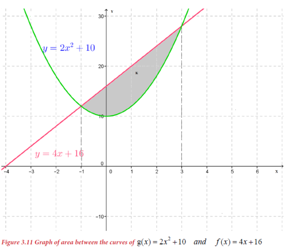
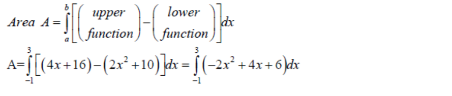
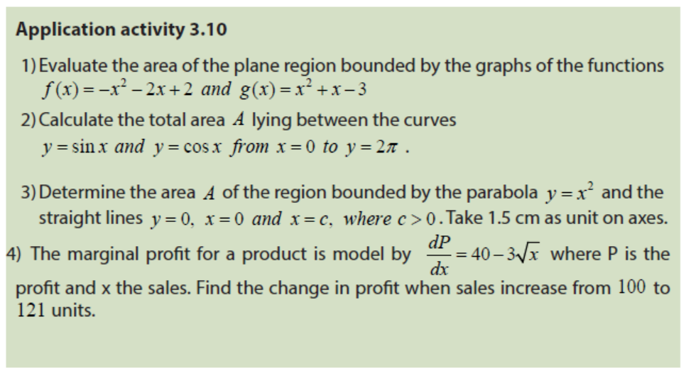
Use integration as an inverse of differentiation and then apply definite integrals tofind area of plane shapes.
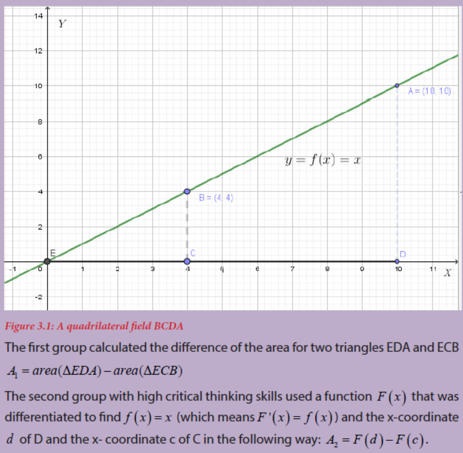
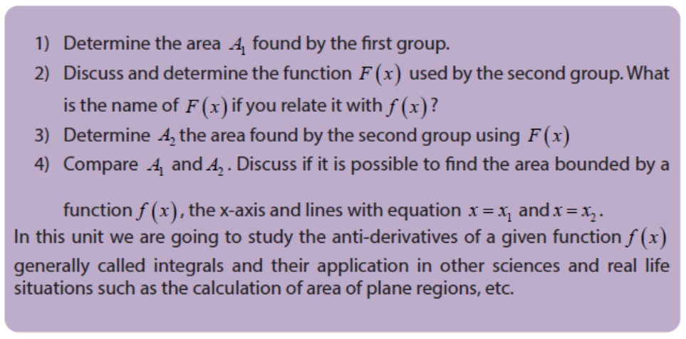
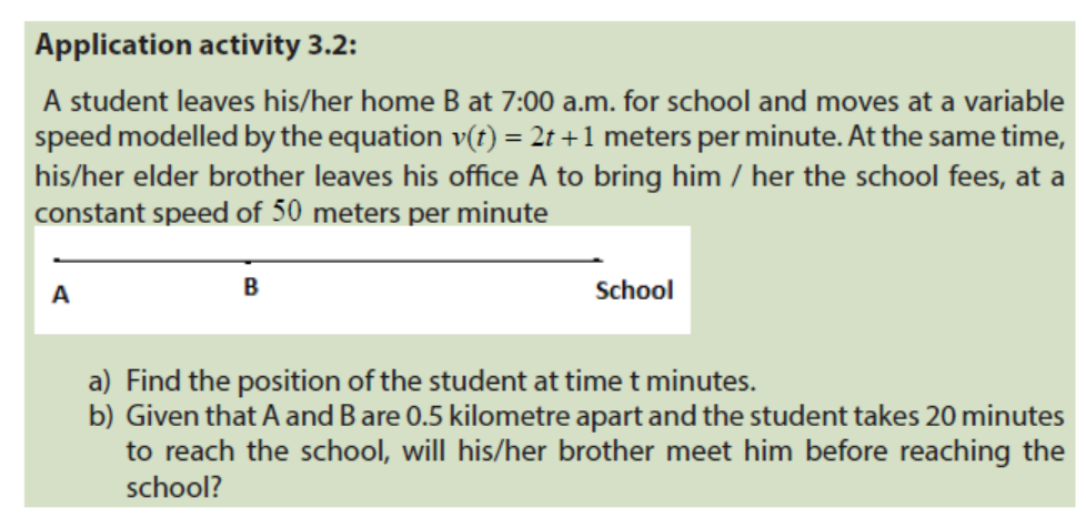
Introductory activity
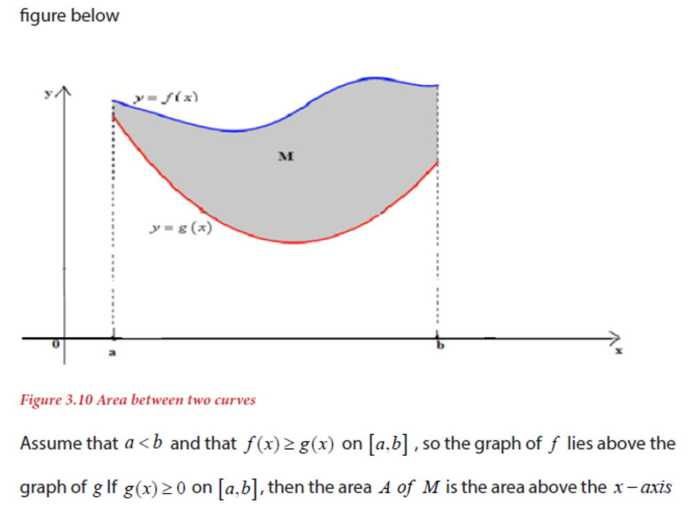
Two groups of students were asked to calculate the area of a quadrilateral fieldBCDA shown in the following figure:
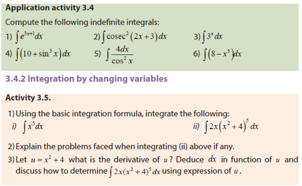
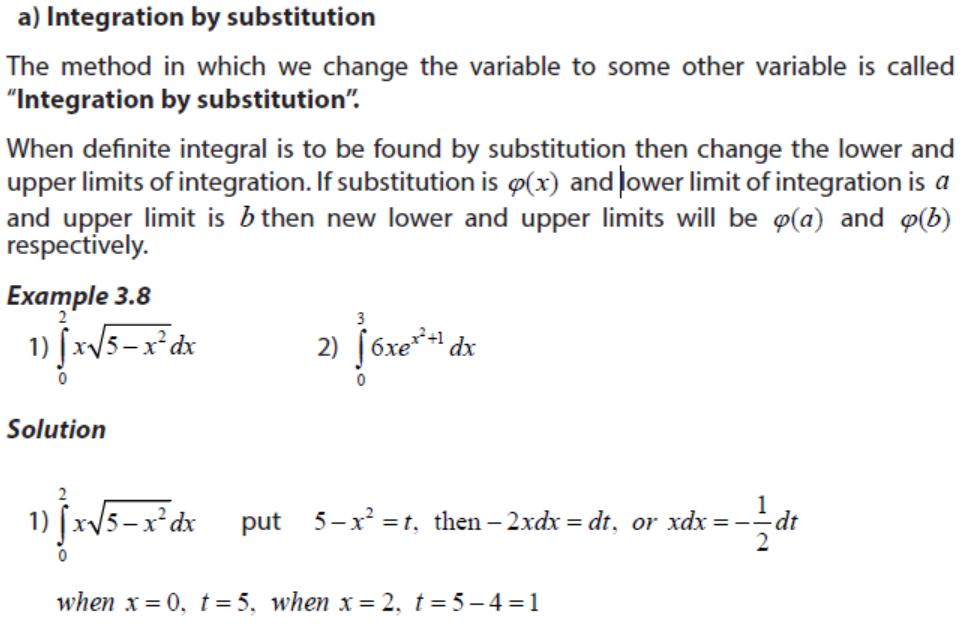
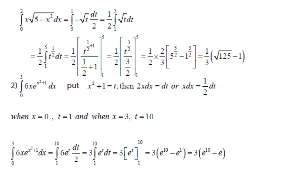
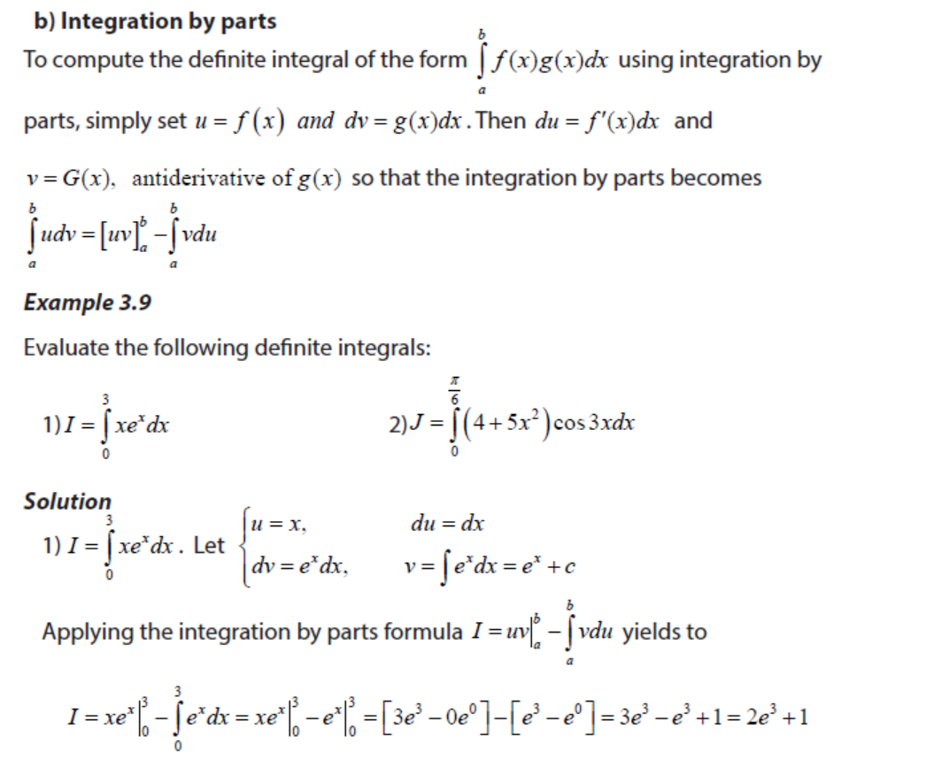
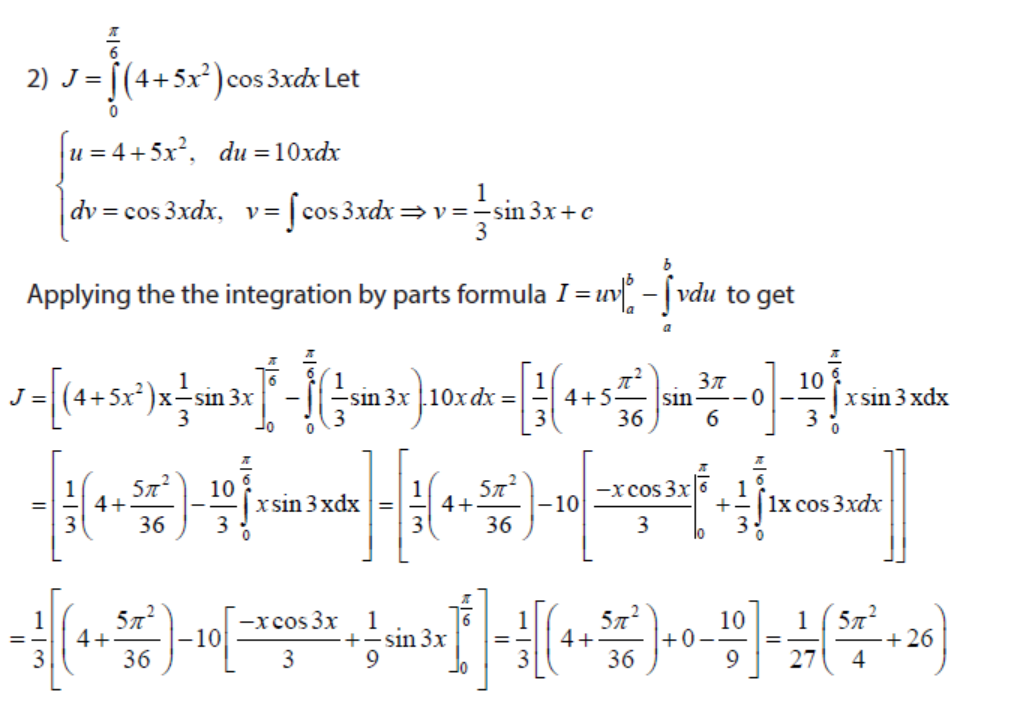
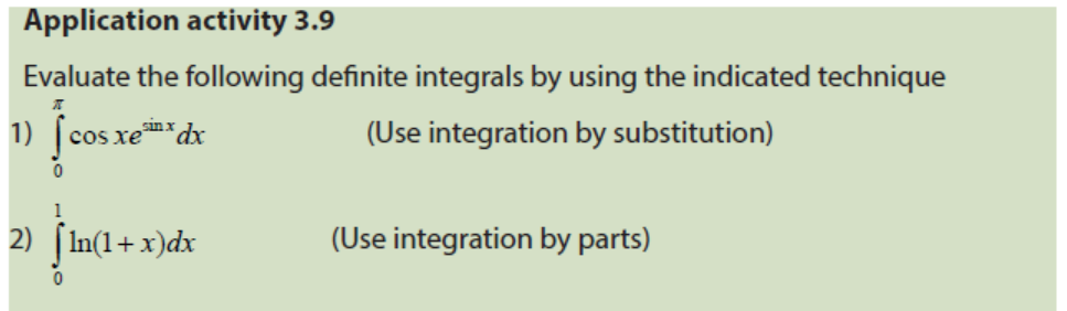
3.4.3 Integration by parts
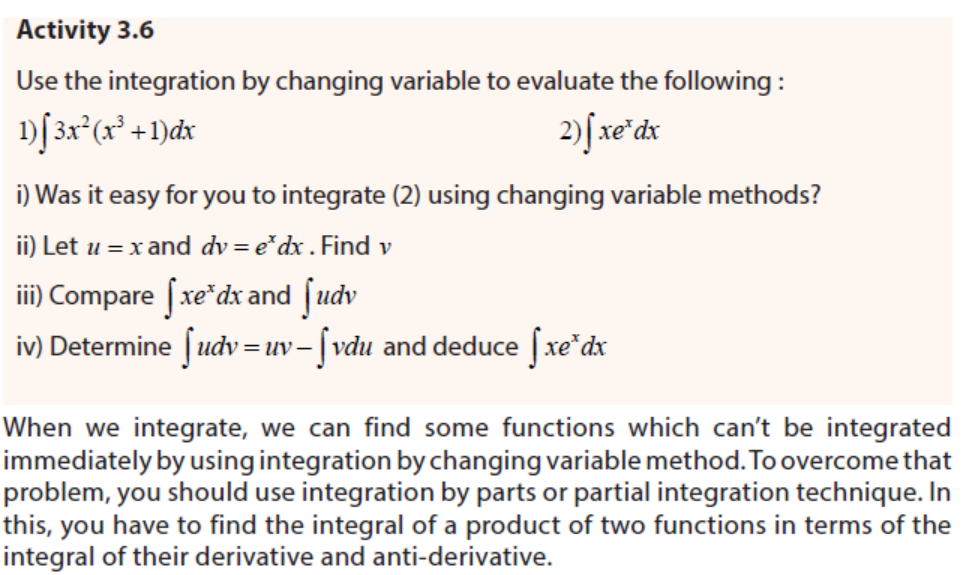
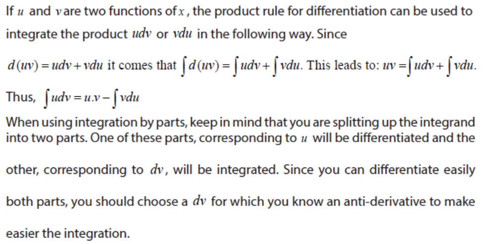
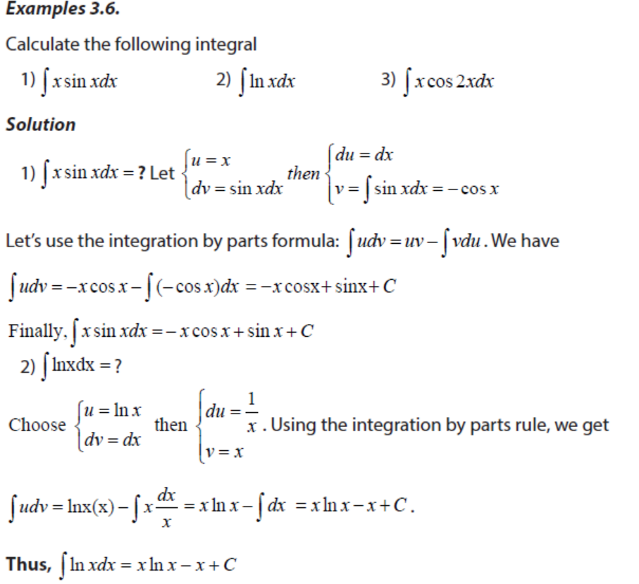
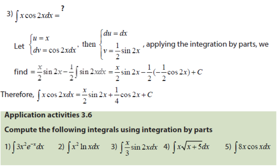


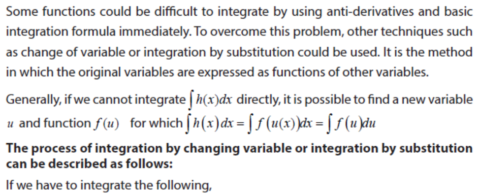
 Many times, some functions can not be integrated directly. In that case we have
to adopt other techniques in finding the integrals. The fundamental theorem in
calculus tells us that computing definite integral of f(x) requires determining its
antiderivtive, therefore the techniques used in determining indefinite integrals arealso used in computing definite integrals.

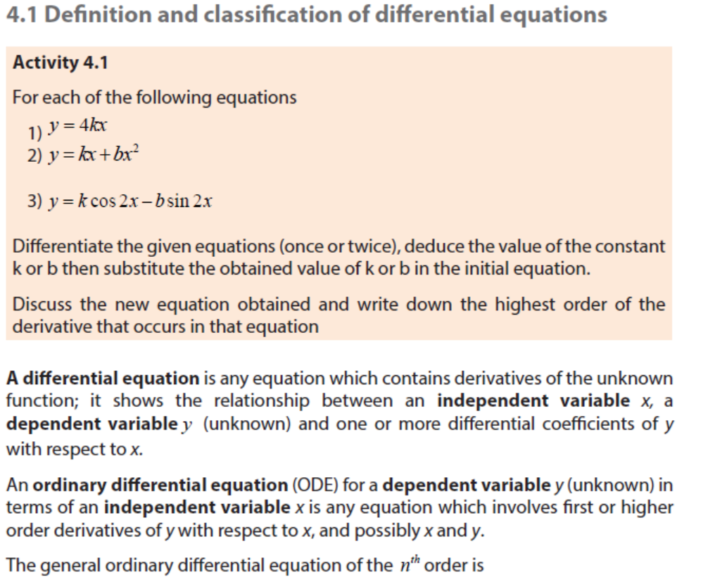
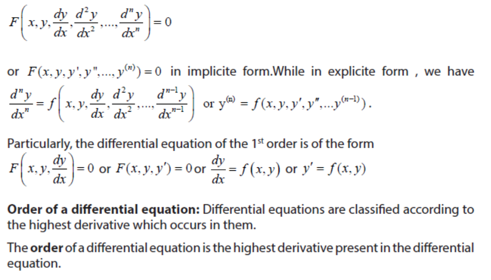
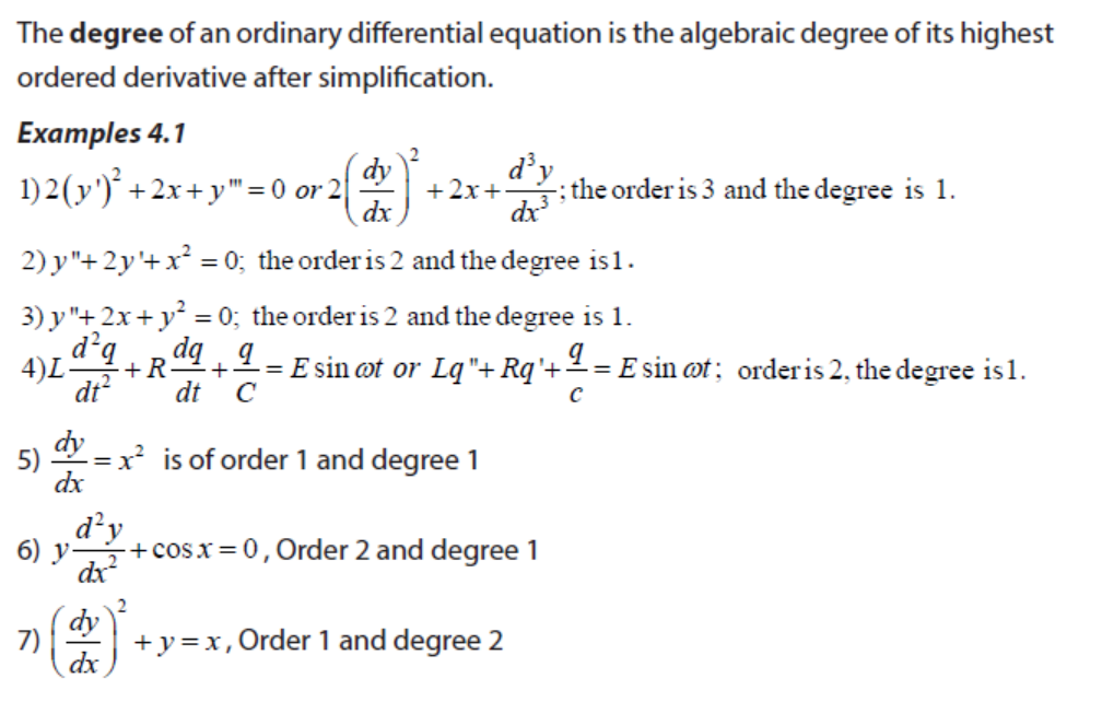
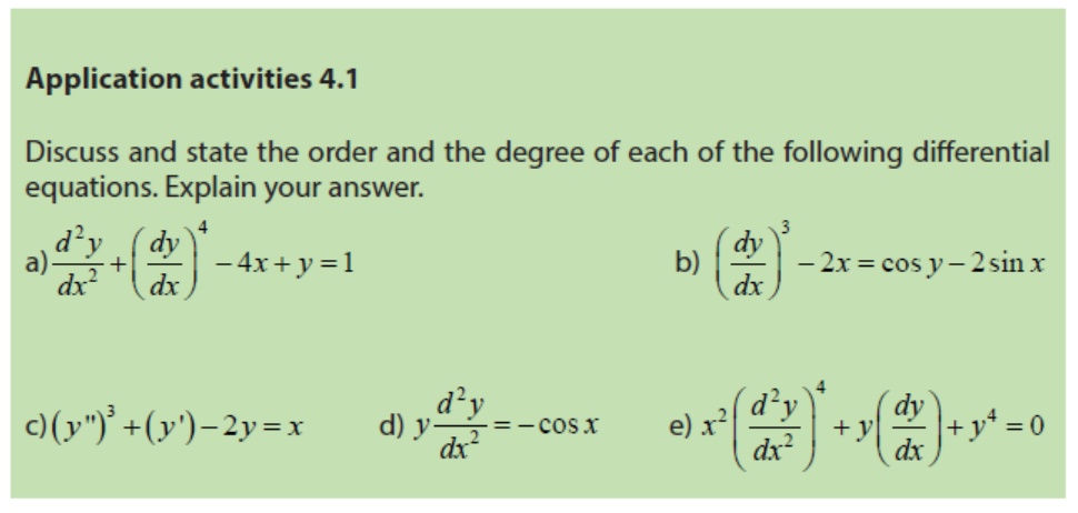
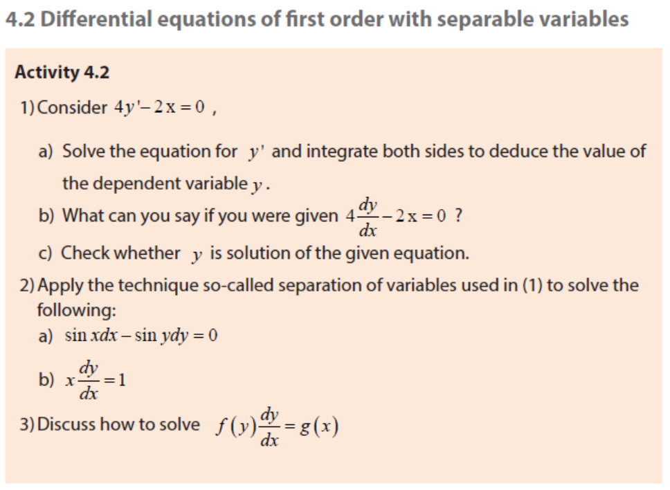
Unit 4. ORDNINARY DIFFERENTIAL EQUATIONS
Unit 4. ORDNINARY DIFFERENTIAL EQUATIONS
Key unit competence
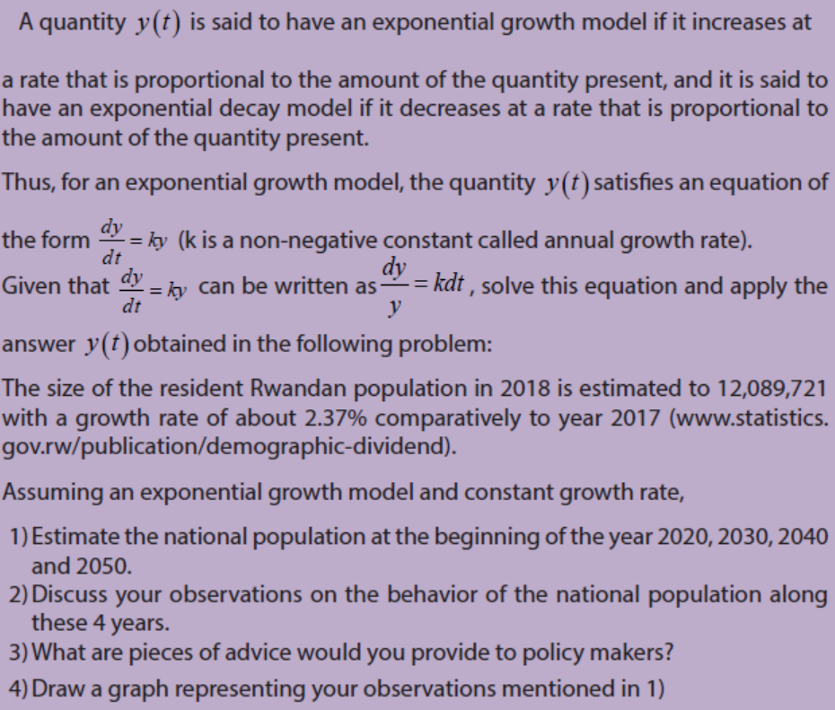
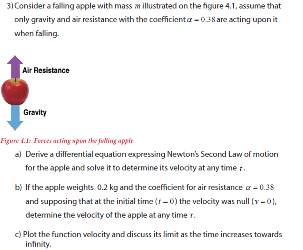
Use ordinary differential equations of first and second order to model and solverelated problems in Physics, Economics, Chemistry, Biology, Demography, etc.

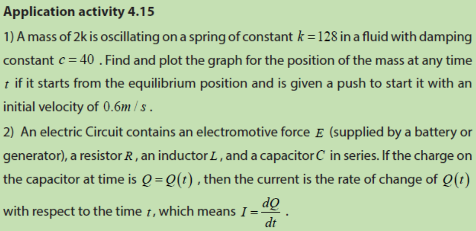
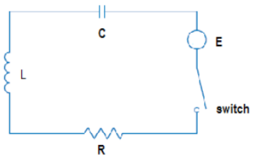
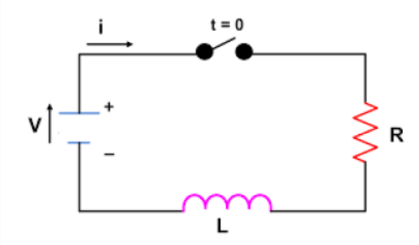
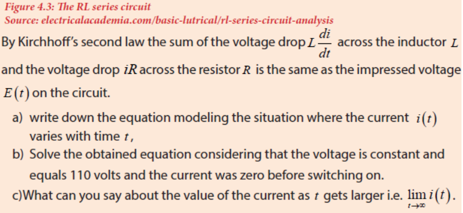
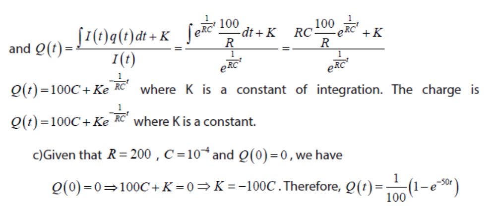
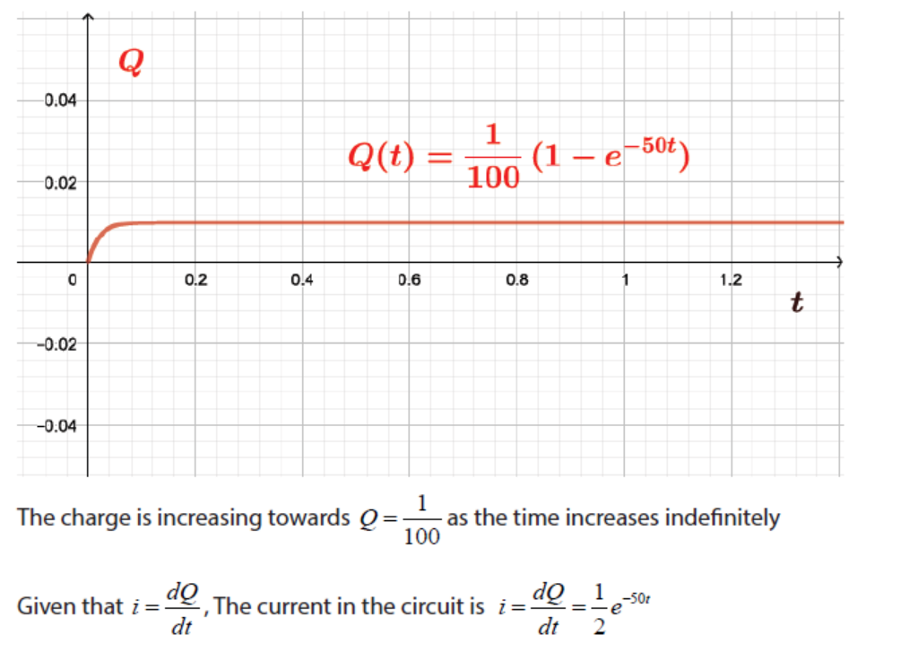
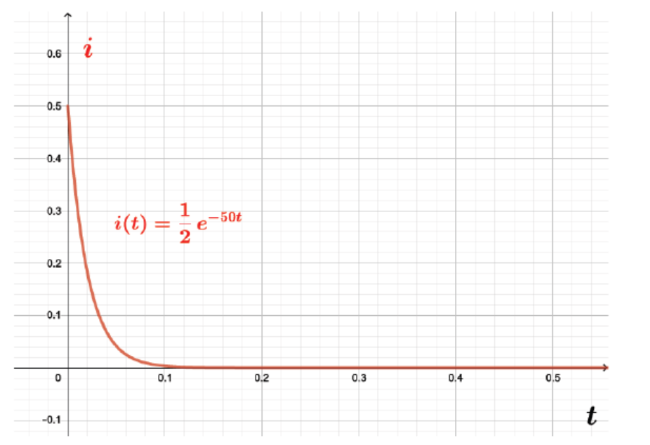
4.4.5 Differential equations in electricity (Series Circuits)
Activity 4.8
Let a series circuit contain only a resistor and an inductor as shown in Figure 4.3

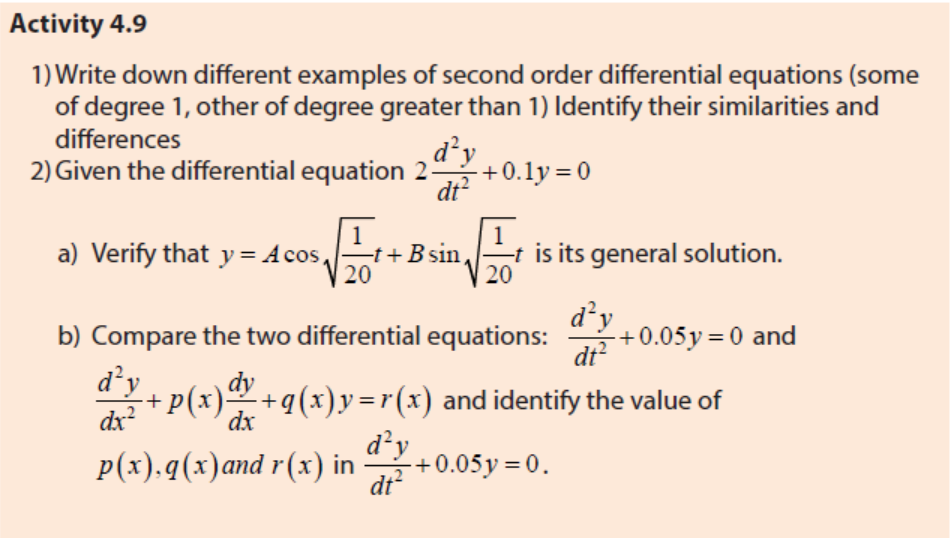
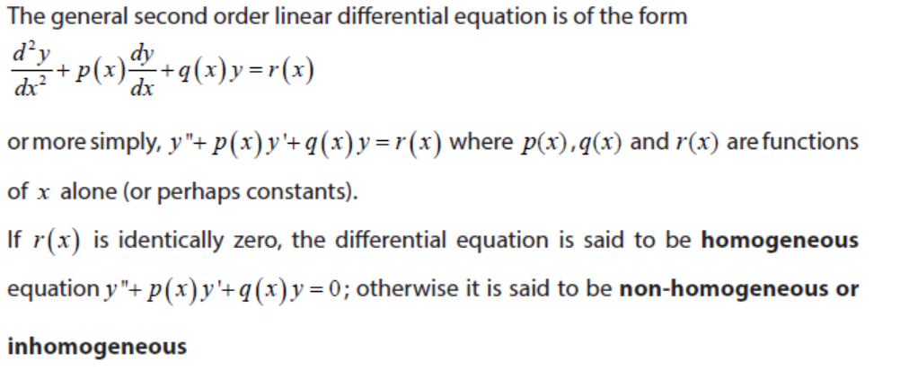
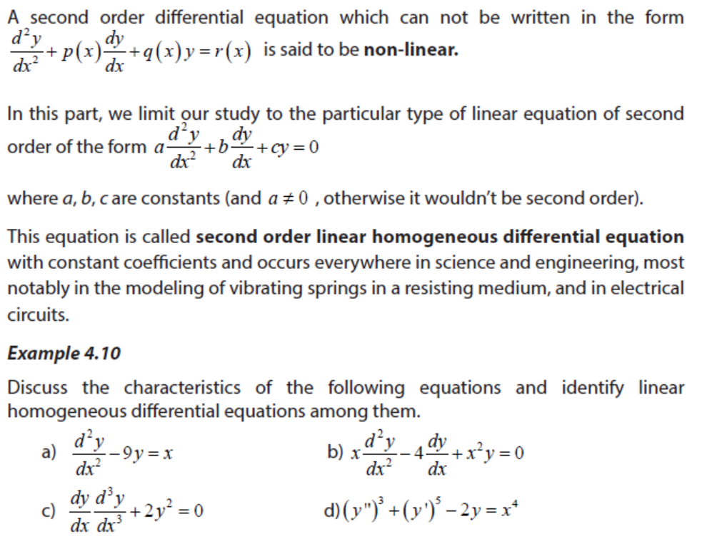
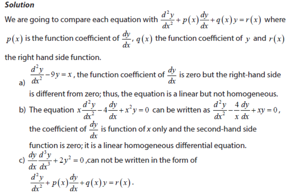
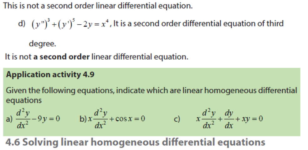
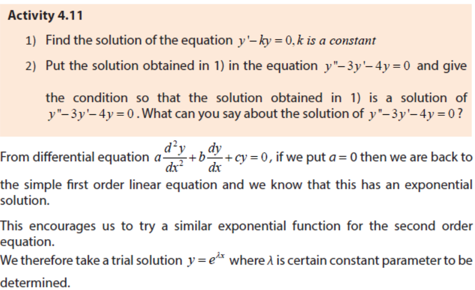
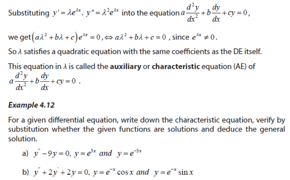
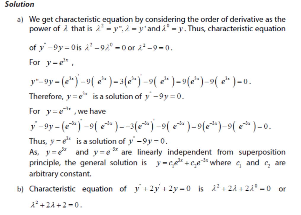
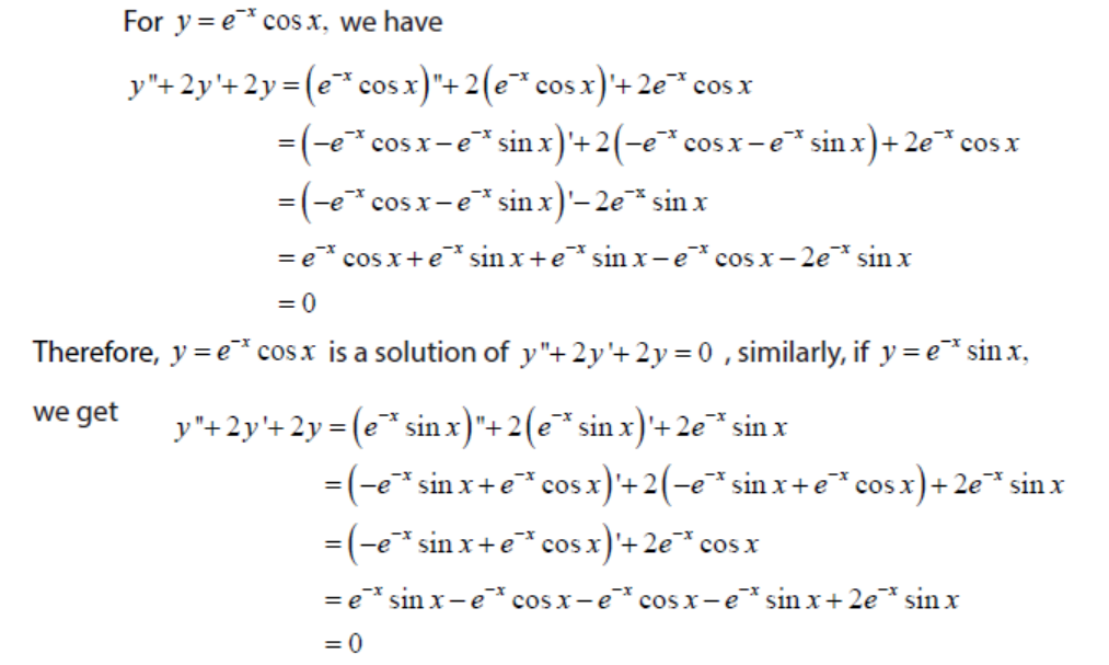
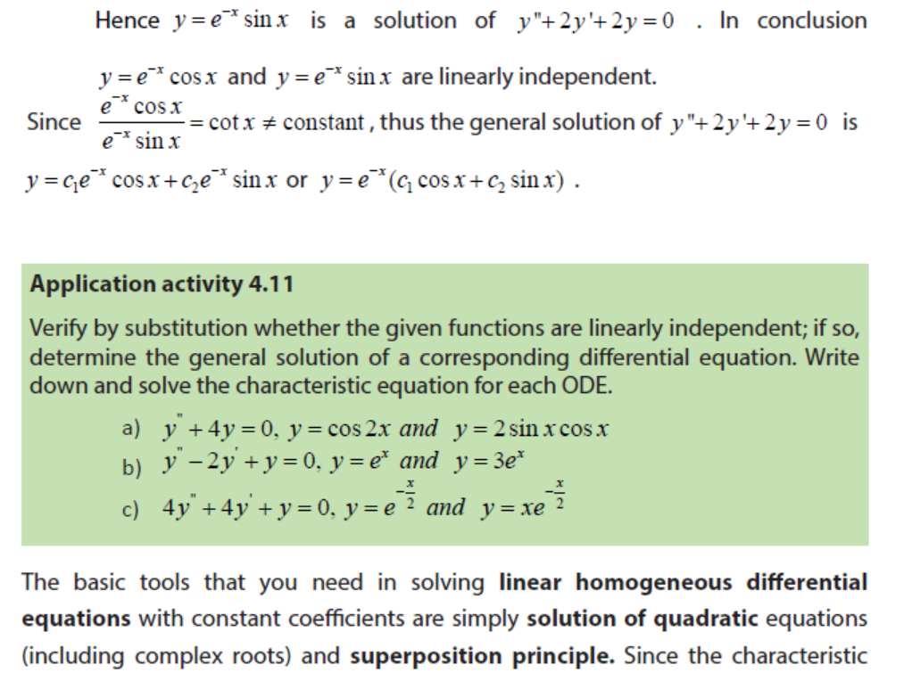
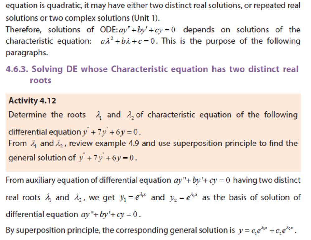
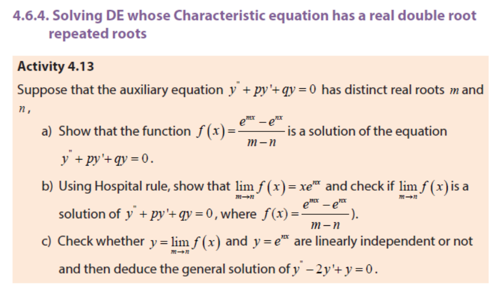
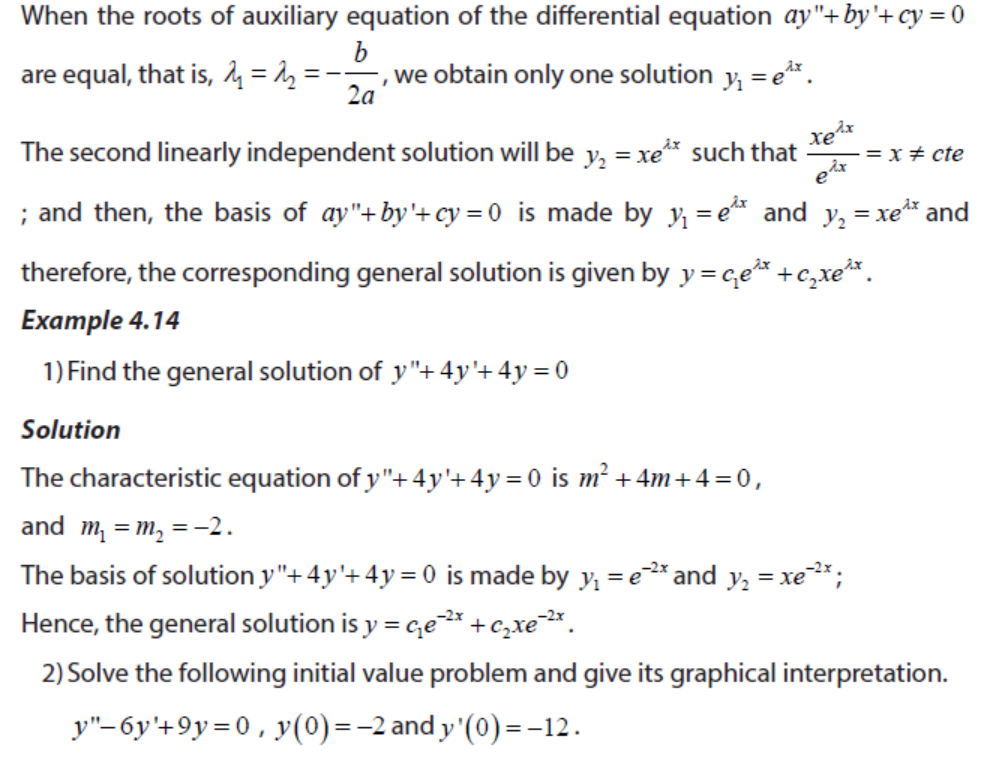
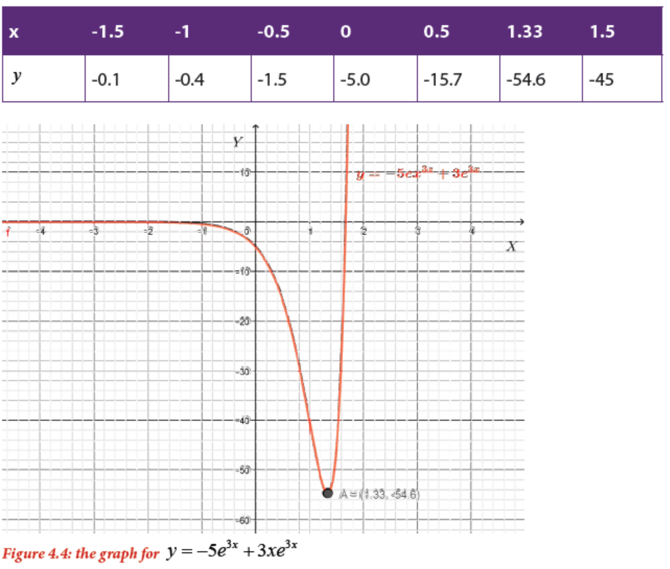
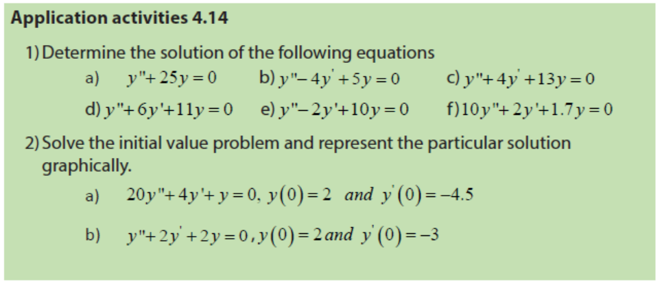
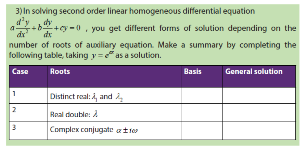
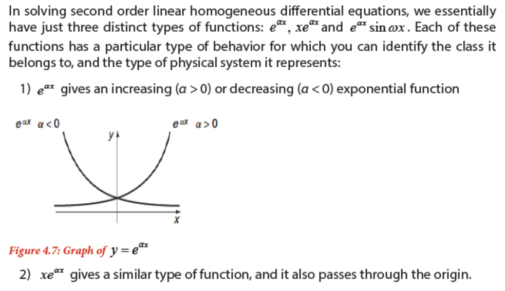
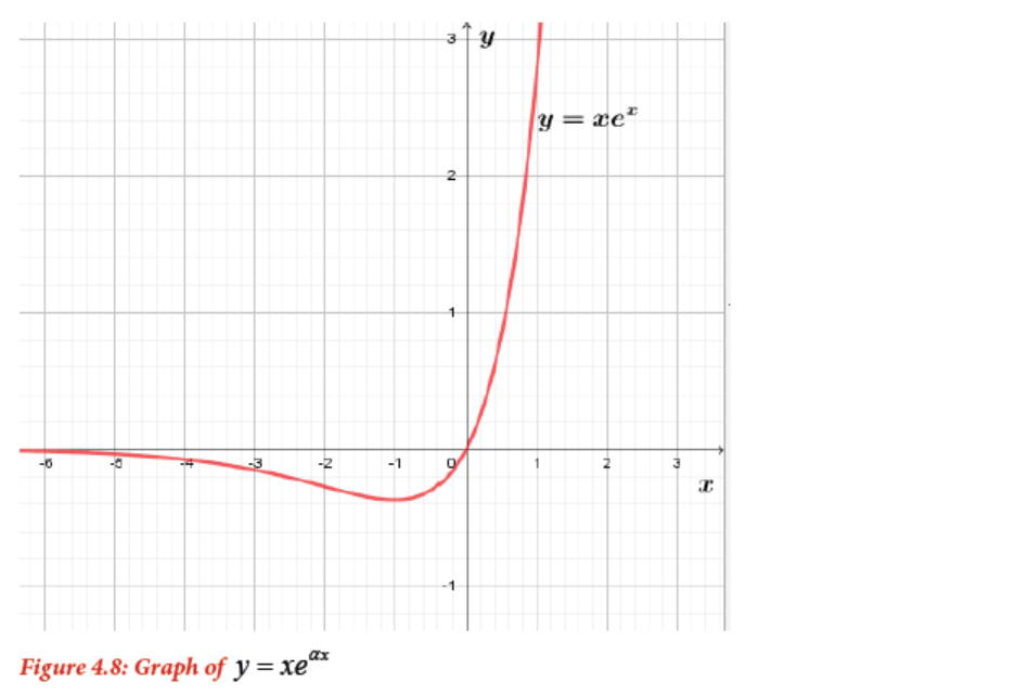
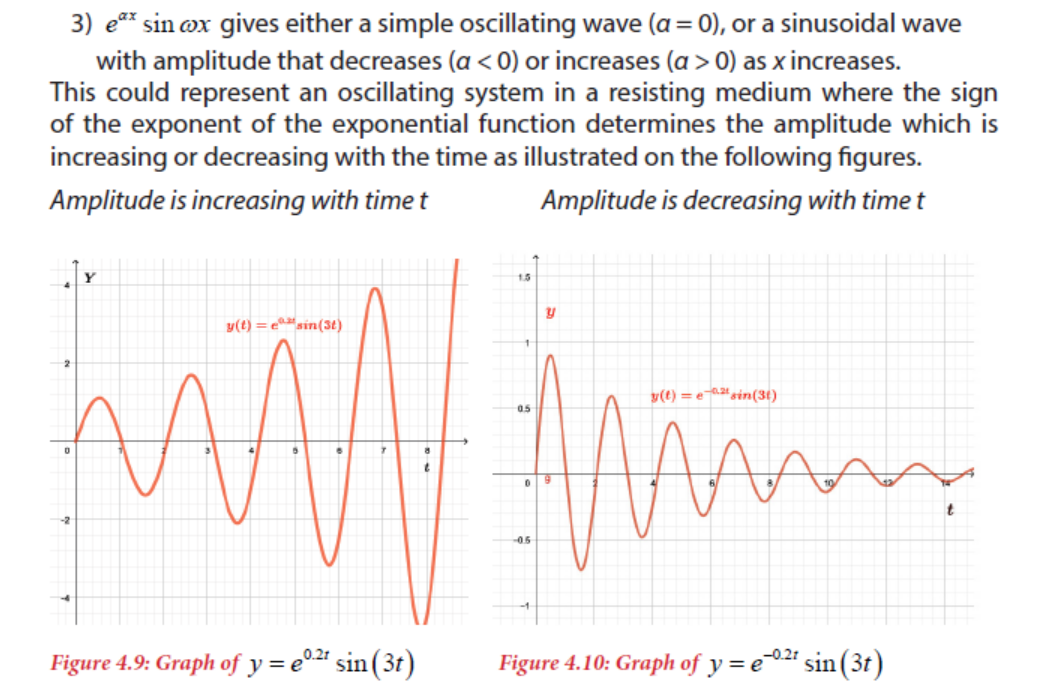
4.5. Introduction to second order linear homogeneous ordinary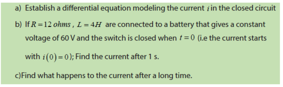
differential equations