General
- Mathematics TG LE Year 2 File Uploaded 16/11/20, 11:10
- Mathematics SB LE Year 2 File Uploaded 16/11/20, 11:07
UNIT 1:FUNCTIONS AND GRAPHS
Key unit Competence: Apply graphical representation of function in economics models
1.0 INTRODUCTORY ACTIVITY
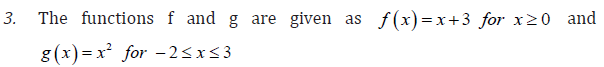
1.1. Generalities on numerical functions
ACTIVITY 1.1
Content summary
1.1.1 Function
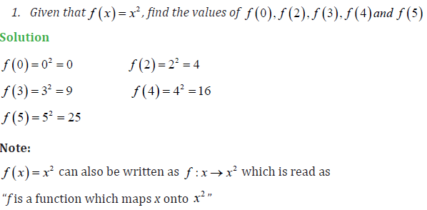
A function is a rule that assigns to each element in a set A one and only one element in set B. We can even define a function as any relationship which takes one element of one set and assigns to it one and only one element of second set.
Examples
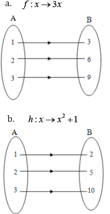
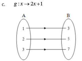
2. Draw arrow diagrams for the functions. Use the domain {1,2,3}
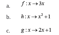
Solution
State the range of each of these functions.
Solution
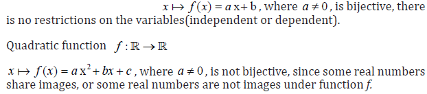
1.1.2 Injective, surjective and bijective functions
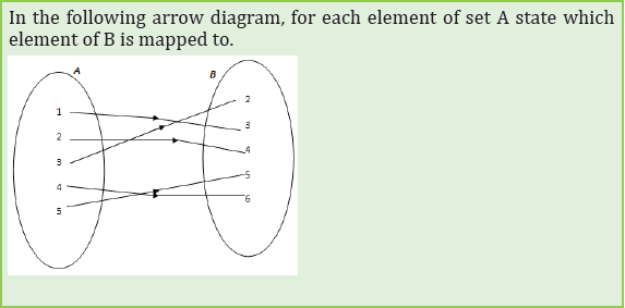
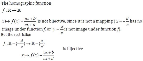
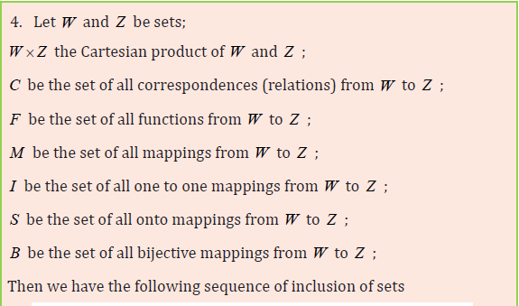
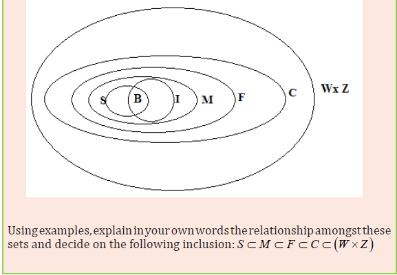
Given sets A and B, a function defined from A to B is a correspondence, or a rule that associates to any element of A either one image in B, or no image in B.
A function such that every elements of A has an image in B is called a mapping, thus, under a mapping any element of A has exactly one image in B (not less than one, and not more than one).
A mapping such that every element of B is image of either one element of A, or of no element of A, is called a one- to- one mapping, or an injective mapping or simply an injection; under a one-to-one mapping no two elements of A share the common image in B.

A mapping such that every element of B is image of at least one element of A (image of one element of A, or image of more than one element of A), is called an onto mapping, or a surjective mapping or simply a surjection

A mapping satisfying properties of both one-to-one and onto is said to be a bijective mapping, or simply a bijection.

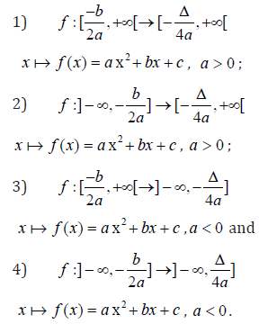
But the following restrictions are bijective:
Examples:
1) Consider the set of pigeons and the set of pigeonholes on the diagram below to answer the questions:
Determine whether it can be established or not between the two sets:
a. A mapping,
b. A one-to-one mapping,
c. An onto mapping,
d. A bijective mapping:
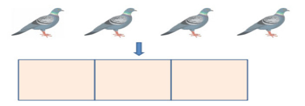
Solution:
Let the pigeons be numbered a, b, c, d and the pigeonholes be numbered 1,2,3.
a. It is possible to establish a mapping between the two sets. For example,
{(a,1);(b, 2);(c,3);(d,3)}.This function is a mapping since each pigeon is accommodated in exactly one pigeonhole, though pigeons c and d are in the same pigeonhole.
b. It is not possible to establish a one-to-one mapping, since sharing images is not allowed. A function from one finite set to a smaller finite set cannot be one-to-one: there must be at least two elements that have the same image
c. The example given in part (a) illustrates a mapping that is onto: no pigeonhole is empty.
d. It is impossible to define a bijection, since it is already impossible to establish a one-to-one mapping
a. One-to-one
b. Onto
c. Bijective.
Solution:
Solution
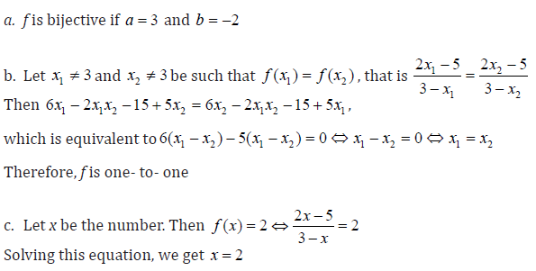
is bijective
a. Find the values of a and b
b. Show that f is one-to-one
c. Find the real number whose image is 2
Solution:
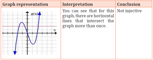
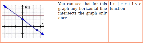
Horizontal Line Test
Horizontal Line Test states that a function is a one to one(injective) function if
there is no horizontal line that intersects the graph of the function at more than one point.
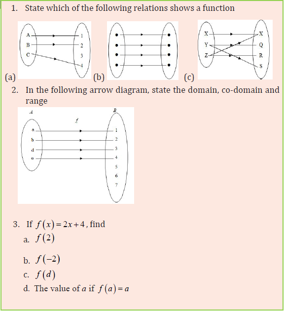
APPLICATION ACTIVITY 1.1
1.2 Types of numerical functions
ACTIVITY 1.2
a) Constant function
A function that assigns the same value to every member of its domain is called a constant function.
This is
 c where c is a given real number.
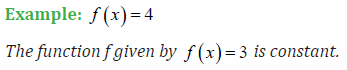
Remark
The constant function that assigns the value c to each real number is sometimes
called the constant function c.
b) Identity: The identity function is of the form

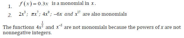
c) Monomial
A function of the form cxn , where c is constant and n a nonnegative integer is called a monomial in x.
Examples
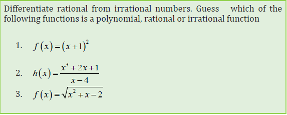
d) Polynomial
A function that is expressible as the sum of finitely many monomials in x is called
Polynomial in x.
Examples:
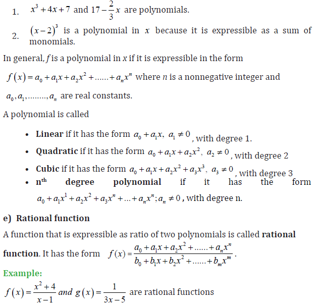
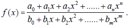
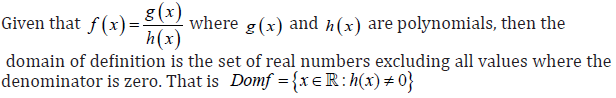
e) Rational function
A function that is expressible as ratio of two polynomials is called rational
function. It has the form
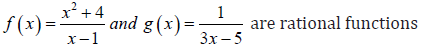
Example:
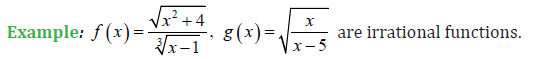
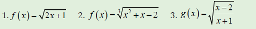
f) Irrational function
A function that is expressed as root extractions is called irrational function.

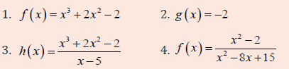
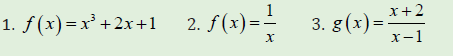
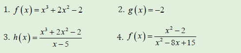
APPLICATION ACTIVITY 1.2
What is the type of the following function?
5. Provide other types of functions and explain your reasons with examples
1.3 Domain of definition for a numerical function
ACTIVITY 1.3.1
For which value(s) the following functions are not defined
ACTIVITY 1.3.2
Find the domain of definition for each of the following functions
ACTIVITY 1.3.3
For each of the following functions, give a range of values of the variable x for which the function is not defined
Content summary
(1) Case of polynomial functions
From the graphs, one can observe that each value of x has its corresponding y value.
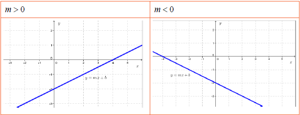
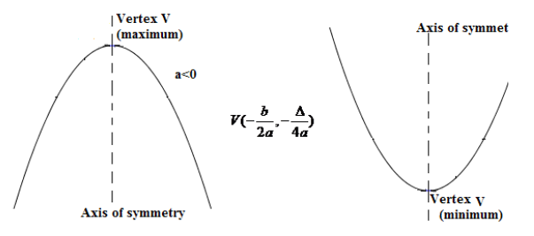
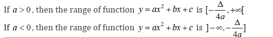
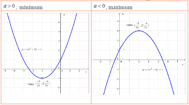
For quadratic functions y = ax2 + bx + c , the main features are summarized on the graph below:
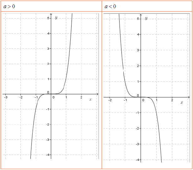
For cubic functions f (x) = ax3 + bx2 + cx + d;a ≠ 0 ,the trends of the graphs are as shown below:
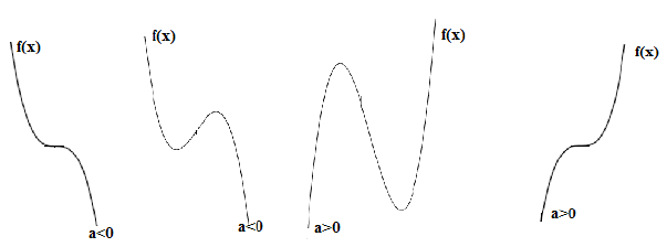
In each case, the domain is ]−∞,+∞[ and the range is ]−∞,+∞[
Even though the range for polynomials of odd degrees is the set of all real numbers, it is not the case for polynomials of even degree greater or equal to 4.
The determination of the range is not easy unless the function is given by its graph; in this case, find by inspection, on the y-axis, the set of all points such that the horizontal lines through those points cut the graph.
Example
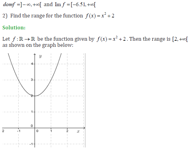
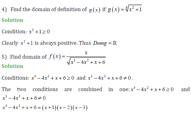
1) Determine the domain and range of
 shown on the graph below:
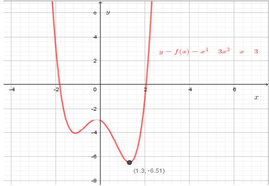
Solution:
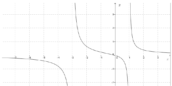
(2) Case for rational functions
Example
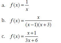
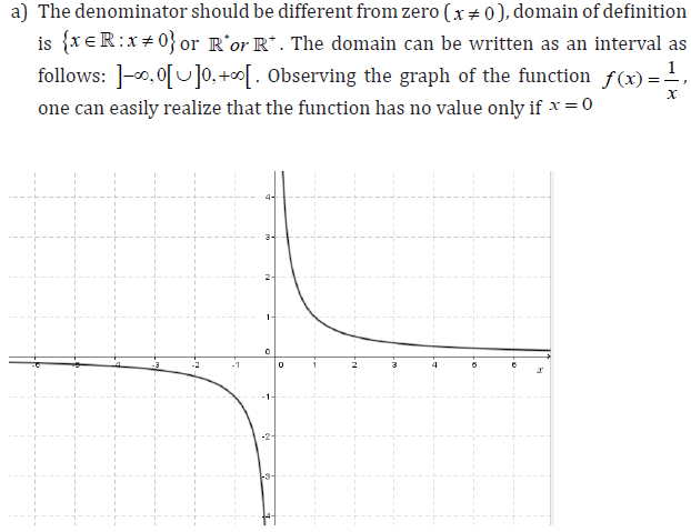
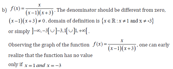
1) Find the domain of each of the functions:
Solution
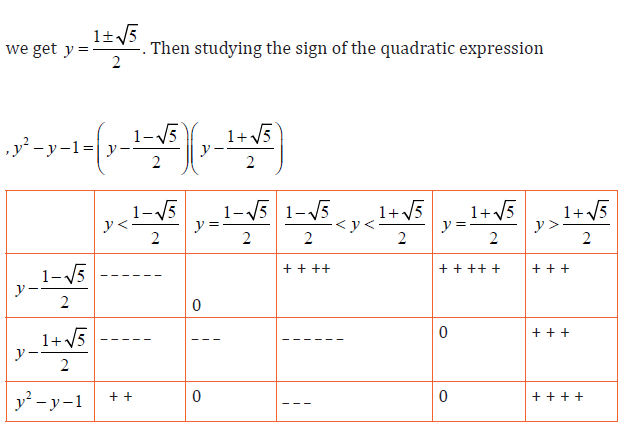
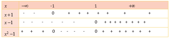
(3) Case for irrational functions
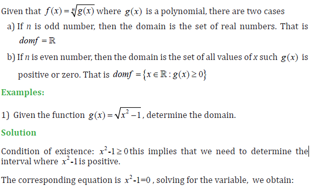
x2 -1=0 Û ( x -1)( x +1) =0
x -1 = 0 Þ x = 1
x + 1 = 0 Þ x = -1

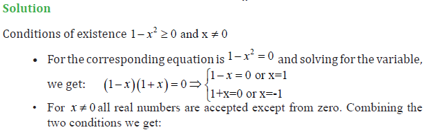
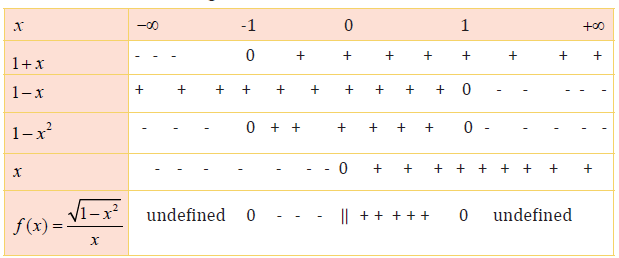
Solution
Since the index in radical sign is odd number, then

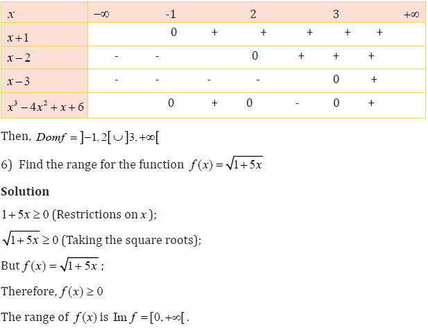
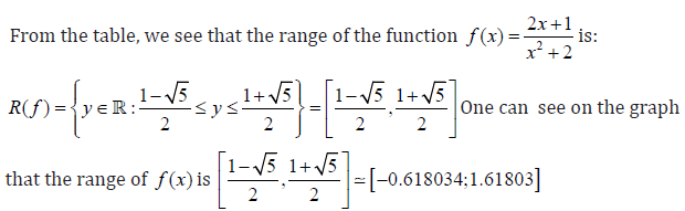
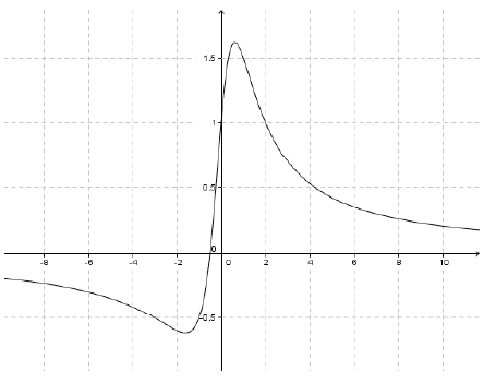
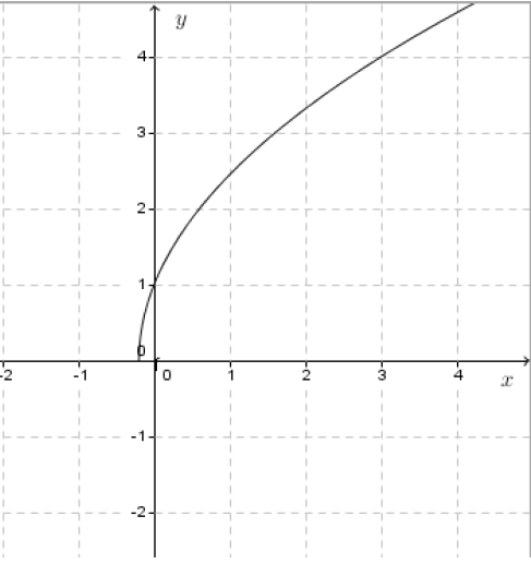
The graph below illustrates the range:
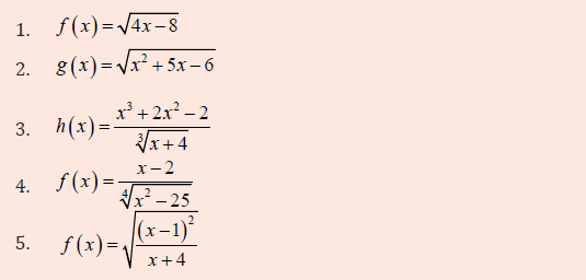
APPLICATION ACTIVITY 1.3
Find the domain of definition for each of the following functions
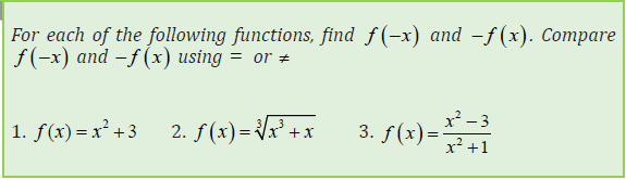
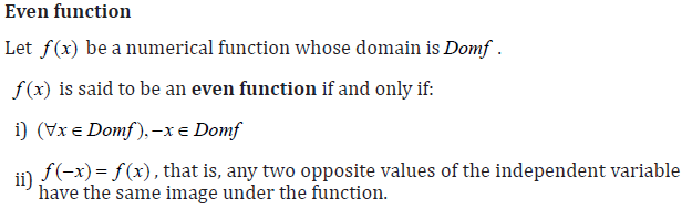
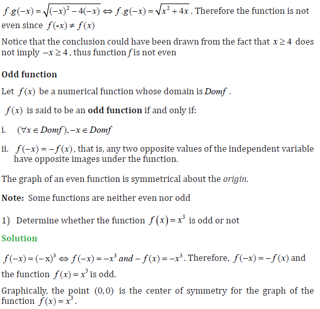
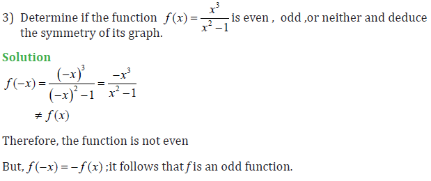
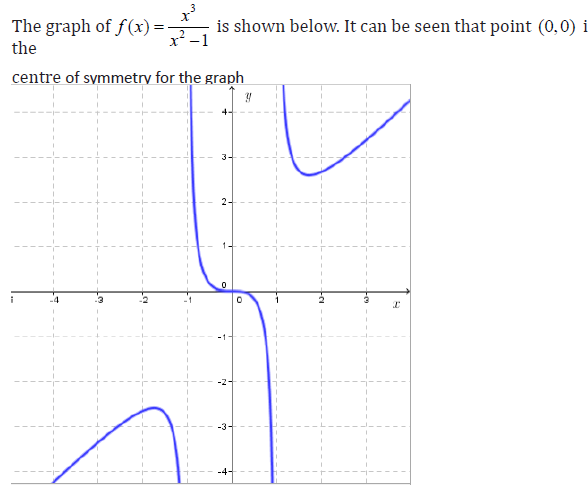
1.4 Parity of a function (odd or even)
ACTIVITY 1.4
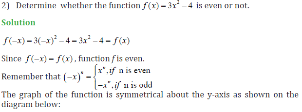
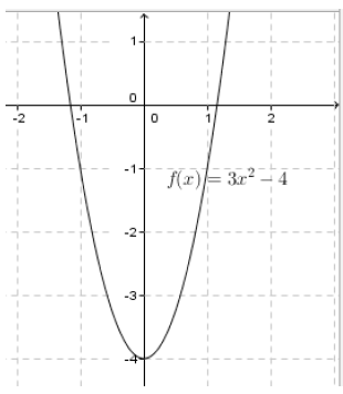
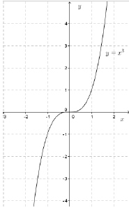
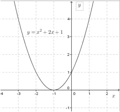
The graph of an even function is symmetrical about the y-axis.
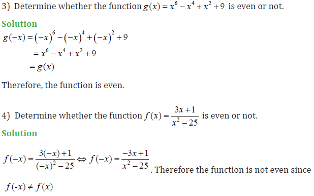
Examples

Solution
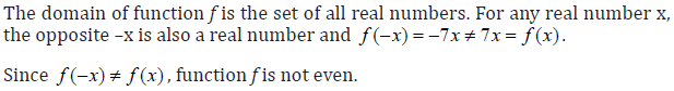
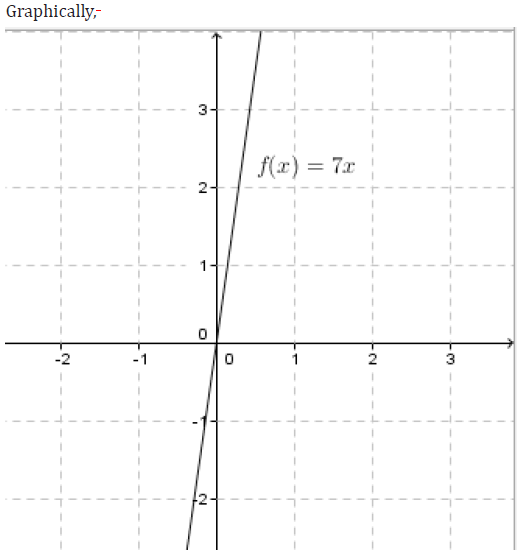
The graph is not symmetrical about the y-axis
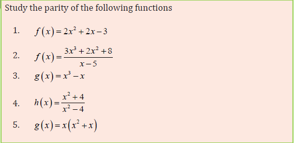
APPLICATION ACTIVITY 1.4
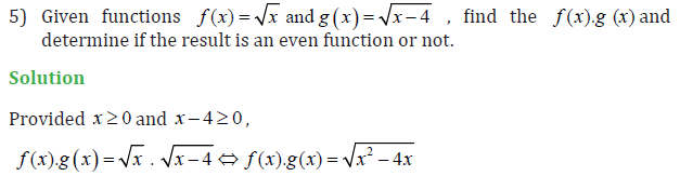
1.5 Operations on functions
1.5.1 Addition, subtraction, multiplication and division
LEARNING ACTIVITY 1.5.1
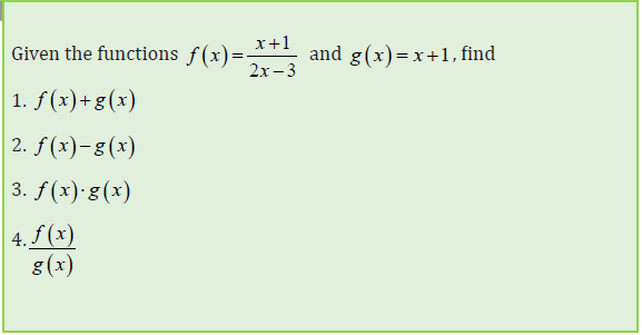
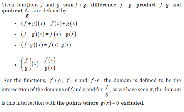
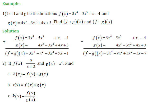
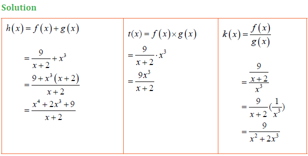
Just as numbers can be added, subtract, multiplied and divided to produce other numbers, there is a useful way of adding, subtracting, multiplying and dividing functions to produce other functions. These operations are defined as follows:
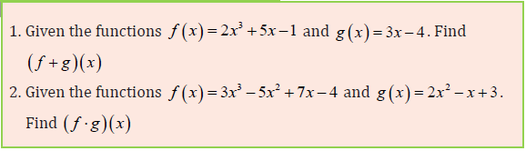
APPLICATION ACTIVITY 1.5.1
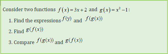
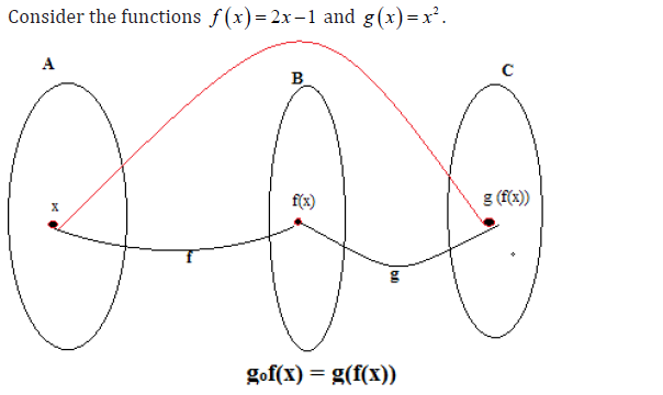
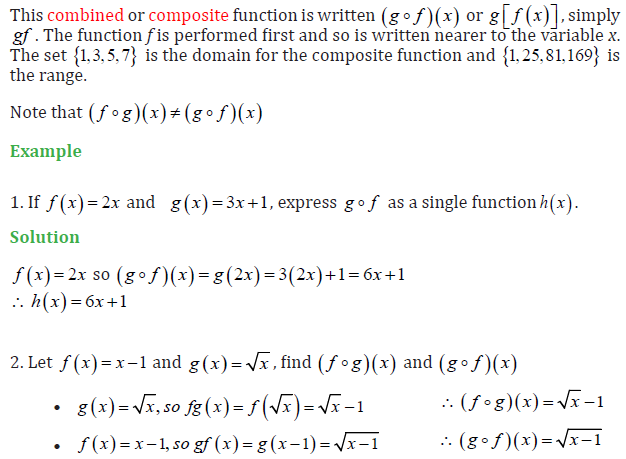
1.5.2 Composite functions
ACTIVITY 1.5.2
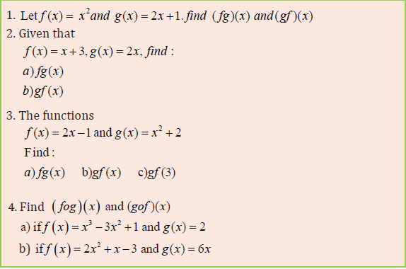
APPLICATION ACTIVITY 1.5.2
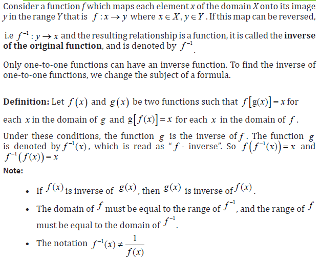
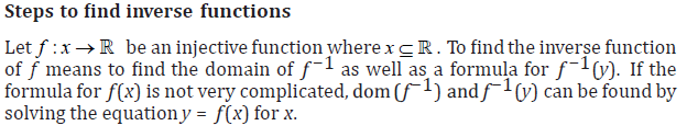
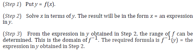
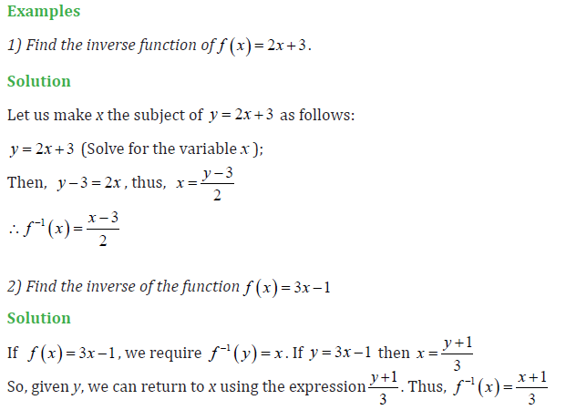
1.5.3 The inverse of a function
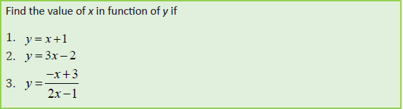
ACTIVITY 1.5.3
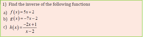
APPLICATION ACTIVITY 1.5.3
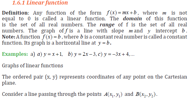
1.6 Graphical representation and interpretation of linear and quadratic functions
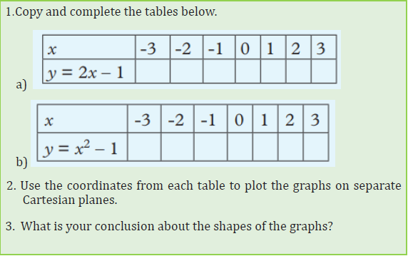
ACTIVITY 1.6
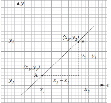
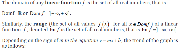
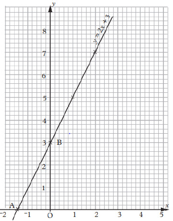
When drawing a graph of a linear function, it is sufficient to plot only two points and these points may be chosen as the x and y intercepts of the graph.
In practice, however, it is wise to plot three points. If the three points lie on the same line, the working is probably correct, if not you have a chance to check whether there could be an error in your calculation.
If we assign x any value, we can easily calculate the corresponding value of y.
For convenience and ease while reading, the calculations are usually tabulated
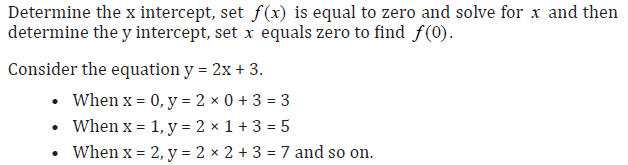
as shown below in the table of values for y = 2x + 3.
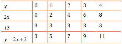
From the table the coordinates (x, y) are (0, 3), (1, 5), (2, 7), (3, 9), (4, 11)....
When drawing the graph, the dependent variable is marked on the vertical axis generally known as the y – axis. The independent variable is marked on the horizontal axis also known as the x – axis.
1.6.2 Quadratic function
A polynomial equation in which the highest power of the variable is 2 is called a quadratic function. The expression y = ax2 + bx + c , where a,b and c are constants and a ≠ 0, is called a quadratic function of x or a function of the second degree (highest power of x is two).
Table of values are used to determine the coordinates that are used to draw thegraph of a quadratic function. To get the table of values, we need to have the domain (values of an independent variable) and then the domain is replaced in a given quadratic function to find range (values of dependent variables). The values obtained are useful for plotting the graph of a quadratic function. All quadratic function graphs are parabolic in nature.
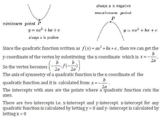
Any quadratic function has a graph which is symmetrical about a line which is parallel to the y-axis i.e. a line x = h where h is constant value. This line is called axis of symmetry.

For any quadratic function f (x) = ax2 + bx + c whose axis of symmetry is the line x = h , the vertex is the point (h, f
).
The vertex of a quadratic function is the point where the function crosses its axis of symmetry.
If the coefficient of the x2 term is positive, the vertex will be the lowest point on the graph, the point at the bottom of the U-shape. If the coefficient of the term x2 is negative, the vertex will be the highest point on the graph, the point at the top of the ∩-shape. The shapes are as below.
Graph of a quadratic function
The graph of a quadratic function can be sketched without table of values as
long as the following are known.
- The vertex
- The x-intercepts
- The y-intercept
APPLICATION ACTIVITY 1.6
1.Using the table of values, sketch the graph of the following functions:
a) y = – 3x + 2
b) y = x2 – 3x + 2
2. Without tables of values, state the vertex, intercept with axis, axis of symmetry, and sketch the graph of
−3x2 + 6x +1 = y
1.7 Graphical representation and interpretation of functions in economics and finance
ACTIVITY 1.7
Content summary
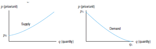
1. Price as function of quantity supplied
The quantity q of an item that is manufactured and sold depends on its price p
As the price increases, manufacturers are usually willing to supply more of the
product, whereas the quantity demanded by consumers falls.
The supply curve, for a given item, relates the quantity q of the item that
manufacturers are willing to make per unit time to the price p for which the item can be sold.
The demand curve relates the quantity q of an item demanded by consumers per unit time to the price p of the item.
Economists often think of the quantities supplied and demanded Q as functions of price P. However, for historical reasons, the economists put price (the independent variable) on the vertical axis and quantity (the dependent variable) on the horizontal axis. (The reason for this state of affairs is that economists originally took price to be the dependent variable and put it on the vertical axis
Theoretically, it does not matter which axis is used to measure which variable.
However, one of the main reasons for using graphs is to make analysis clearer to understand. Therefore, if one always has to keep checking which axis measures which variable this defeats the objective of the exercise. Thus, even though it may upset some mathematical purists, the economists sometimes stick to the convention of measuring quantity on the horizontal axis and price on the vertical axis, even if price is the independent variable in a function.
This means that care has to be taken when performing certain operations on functions. If necessary, one can transform monotonic functions to obtain the inverse function (as already explained) if this helps the analysis.
Examples
This figure shows that when the quantity Q is increasing, the price P reduces progressively.
This can be caused by the fact that every consumer has sufficient quantity of goods and does not want to by any more.
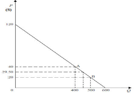
2) Suppose that a firm faces a linear demand schedule and that 400 units of output Q are sold when price is $40 and 500 units are sold when price is $20. Once these two price and quantity combinations have been marked as points A and B, then the rest of the demand schedule can be drawn in. Use this data to determine the function that can help to predict quantities demanded at different prices and draw the corresponding graph.
Solution:
Accurate predictions of quantities demanded at different prices can be made if the information that is initially given is used to determine the algebraic format of the function.
A linear demand function must be in the form P = a − bQ , where a and b are parameters that we wish to determine the value of.
When P = 40 then Q = 400 and so 40 = a − 400b (1)
When P = 20 then Q = 500 and so 20 = a − 500b (2)
Equations (1) and (2) are what is known as simultaneous linear equations.
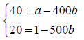
We can solve these simultaneous linear equations by one of the methods we used above and find
a =120, b = 0.02 .
Our function can now be written as P = 120 − 0.2Q
We can check that this is correct by substituting the original values of Q into the function.
If Q = 400 then P = 120 − 0.2(400) = 120 − 80 = 40
If Q = 500 then P = 120 − 0.2(500) = 120 − 100 = 20
These are the values of P originally specified and so we can be satisfied that the
line that passes through points A and B is the linear function P = 120 − 0.2Q.
The inverse of this function will be Q = 600−5P. Precise values of Q can now
be derived for given values of P. For example, when P = £29.50 then Q = 600 −
5(29.50) = 452.5.
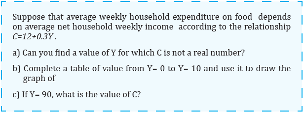
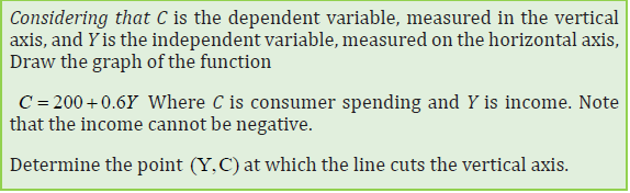
It is assumed that consumption C depends on income Y and that this relationship
takes the form of the linear function C = a + bY .
Example:
When the income is $600, the consumption observed is $660. When the income is $1,000, the consumption observed is $900. Determine the equation “consumption function of income”.
Solution:
To determine the required equation, we can solve this system of equations
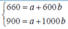
by using different methods to find the value of a and b .
However, let us use another way as follows: We expect b to be positive, i.e. consumption increases with income, and so our function will slope upwards. As this is a linear function then equal changes in Y will cause the same changes in C.
A decrease in Y of $400, from $1,000 to $600, causes C to fall by $240, from $900 to $660.
If Y is decreased by a further $600 (i.e. to zero) then the corresponding fall in
C will be 1.5 times the fall caused by an income decrease of $400, since $600 = 1.5 × $400.
Therefore, the fall in C is 1.5 × $240 = $360. This means that the value of C when
Y is zero is $660 − $360 = $300. Thus a = 300.
A rise in Y of $400 causes C to rise by $240. Therefore, a rise in Y of $1 will cause
C to rise by $240/400 = $0.6. Thus b = 0.6.
The function can therefore be specified as C = 300 + 0.6Y .
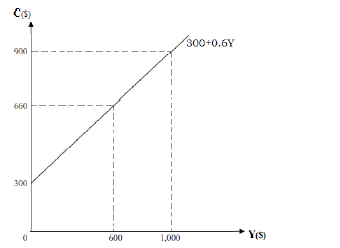
The graph shows that when the income increases, the consumption increases also.
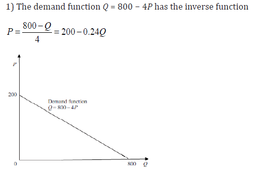
3. Price as function of quantity demanded
The linear demand function is in the form P = a − bQ , where a and b are
parameters, P is the price and Q is the quantity demanded.
Example:
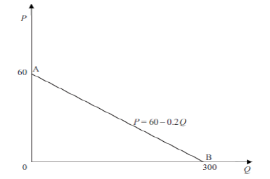
Consider the function P = 60−0.2Q where P is price and Q is quantity demanded.
Assume that P and Q cannot take negative values, determine the slop of this function and sketch its graph.
Solution:
When Q = 0 then P = 60
When P = 0 then 0 = 60 − 0.2Q
Using these points: (0,60) and (300,0) , we can find the graph as follows:
The slope of a function which slopes down from left to right is found by applying the formula
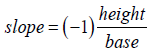
To the relevant right-angled triangle. Thus, using the triangle 0BA, the slope of our function is
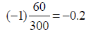
This, of course, is the same as the coefficient of Q in the function P = 60 − 0.2Q.
Remember that in economics the usual convention is to measure P on the vertical axis of a graph. If you are given a function in the format Q = f (P) then you would need to derive the inverse function to read off the slope.
Example:
What is the slope of the demand function Q = 830 − 2.5P when P is measured on the vertical axis of a graph?
Solution:
If Q= 830−2.5P; then 2.5P = 830−Q
P = 332−0.4Q
Therefore, the slope is the coefficient of Q, which is −0.4.
4. Point elasticity of demand
Elasticity can be calculated at a specific point on a linear demand schedule. This
is called ‘point elasticity of demand’ and is defined as
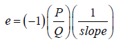
where P and Q are the price and quantity at the point in question. The slope refers to the slope of the demand schedule at this point although, of course, for a linear demand schedule the slope will be the same at all points.
Example:
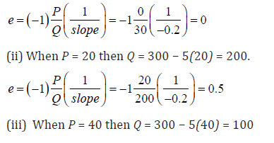
Calculate the point elasticity of demand for the demand schedule P = 60 − 0.2Q where price is
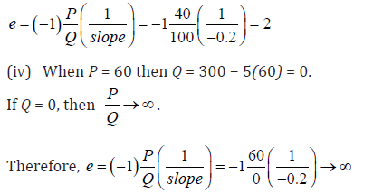
(i) Zero, (ii) $20, (iii) $40, (iv) $60.
Solution
This is the demand schedule referred to earlier and illustrated above. Its slope
must be −0.2 at all points as it is a linear function and this is the coefficient of Q.
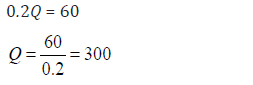
To find the values of Q corresponding to the given prices we need to derive the inverse function. Given that
P = 60 − 0.2Q then 0.2Q = 60 − P
Q = 300 − 5P
(i) When P is zero, at point B, then Q = 300 − 5(0) = 300. The point elasticity will therefore be
5. The Cost Function
The cost function, C(q), gives the total cost of producing a quantity q of some good. Costs of production can be separated into two parts: the fixed costs, which are incurred even if nothing is produced, and the variable costs, which depend on how many units are produced.
Example:
Let’s consider a company that makes radios. The factory and machinery needed to begin production are fixed costs, which are incurred even if no radios are made. The costs of labor and raw materials are variable costs since these quantities depend on how many radios are made. The fixed costs for this company are $24,000 and the variable costs are $7 per radio.
Then, Total costs for the company = Fixed costs + Variable costs = 24,000 + 7.
(Number of radios),
so, if q is the number of radios produced,
C(q) = 24,000 + 7q.
This is the equation of a line with slope 7 and vertical intercept 24,000.
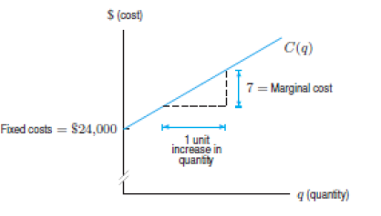
If C(q) is a linear cost function,
- Fixed costs are represented by the vertical intercept.
- Marginal cost is represented by the slope.
6. The Revenue Function
The revenue function, R(q), gives the total revenue received by a firm from selling a quantity, q, of some good.
If the good sells for a price of p per unit, and the quantity sold is q, then Revenue
= Price · Quantity,
so, R = pq.
If the price does not depend on the quantity sold, so p is a constant, the graph
of revenue as a function of q is a line through the origin, with slope equal to the price p.
Example:
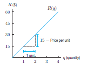
1. If radios sell for $15 each, sketch the manufacturer’s revenue function. Show
the price of a radio on the graph.
Solution:
Since R(q) = pq = 15q, the revenue graph is a line through the origin with a
slope of 15. See the figure. The price is the slope of the line.
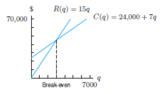
2. Graph the cost function C(q) = 24,000 + 7q and the revenue function R(q) =
15q on the same axes. For what values of q does the company make money?
Solution:
The company makes money whenever revenues are greater than costs, so we
find the values of q for which the graph of R(q) lies above the graph of C(q). See Figure 1.45.
We find the point at which the graphs of R(q) and C(q) cross:
Revenue = Cost
15q = 24,000 + 7q
8q = 24,000
q = 3000.
The company makes a profit if it produces and sells more than 3000 radios. The
company loses money if it produces and sells fewer than 3000 radios.
7. The Profit Function
Decisions are often made by considering the profit, usually written as π to
distinguish it from the price, p .
We have: Profit = Revenue – Cost.
So, π = R −C
The break-even point for a company is the point where the profit is zero and revenue equals cost.
Example:
Find a formula for the profit function of the radio manufacturer. Graph it, marking the break-even point
Solution:
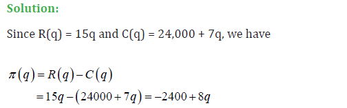
Notice that the negative of the fixed costs is the vertical intercept and the breakeven
point is the horizontal intercept. See the figure;
8. The Marginal Cost, Marginal Revenue, and Marginal Profit
Just as we used the term marginal cost to mean the rate of change, or slope, of a linear cost function, we use the terms marginal revenue and marginal profit to mean the rate of change, or slope, of linear revenue and profit functions, respectively.
The term marginal is used because we are looking at how the cost, revenue, or profit change “at the margin,” that is, by the addition of one more unit.
For example, for the radio manufacturer, the marginal cost is 7 dollars/item (the additional cost of producing one more item is $7), the marginal revenue is 15 dollars/item (the additional revenue from selling one more item is $15), and the marginal profit is 8 dollars/item (the additional profit from selling one more item is $8).
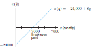
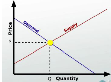
9. Equilibrium Price and Quantity
If we plot the supply and demand curves on the same axes, the graphs cross at the equilibrium point. The values p * and q* at this point are called the equilibrium price and equilibrium quantity, respectively. It is assumed that the market naturally settles to this equilibrium point.
Example:
Find the equilibrium price and quantity if Quantity supplied = 3p − 50 and
Quantity demanded = 100 − 2p.
Solution:
To find the equilibrium price and quantity, we find the point at which
Supply = Demand
3p − 50 = 100 − 2p
5p = 150
p = 30.
The equilibrium price is $30. To find the equilibrium quantity, we use either the demand curve or the supply curve.
At a price of $30, the quantity produced is
100 − 2 (30) = 40 items.
The equilibrium quantity is 40 items.
In the figure, the demand and supply curves intersect at p* = 30 and q* = 40 .
APPLICATION ACTIVITY 1.7
1. Assume that consumption C depends on income Y according to the function
C = a + bY , where a and b are parameters. If C is $60 when Y is $40 and C is $90 when Y is $80,
What are the values of the parameters a and b?
Sketch the graph of C(Y) and interpret it.
2. Suppose that q = f(p) is the demand curve for a product, where p is the
selling price in dollars and q is the quantity sold at that price.
(a) What does the statement f(12) = 60 tell you about demand for this product?
(b) Do you expect this function to be increasing or decreasing? Why?
3. A demand curve is given by 75p + 50q = 300, where p is the price of the product, in dollars, and q is the quantity demanded at that price.
Find p * and q* intercepts and interpret them in terms of consumer demand.
1.8 END UNIT ASSESSMENT
1) The total cost C for units produced by a company is given by
C(q) = 50000 + 8q where q is the number of units produced.
a) What does the number 50000 represent?
b)What does the number 8 represent?
d) Plot the graph of C and indicate the cost when q = 5 .
e) Determine the real domain and the range of C(q) .
f) Is C(q) an odd function?
2) Bosco was working for his boss Kamana and they agreed to start a job where the monthly salary f (t ) was depending on the time t representing the tth month Bosco spends on service. The salary
f (t ) was the sum of a monthly bonus of 50,000Fr and product of 10,000Frw by the inverse of the time t .
a) Give the function f (t ) which models the monthly salary of Bosco;
b) Determine the domain of f (t ) and explain what it means
c) Suppose that Bosco can continue to work indefinitely, determine the Maximum Salary and the Minimum Salary can Bosco get and deduce the Range of f (t ) .
d) Bosco has a monthly bonus, is this bonus motivating? Explain your answer.
e) If you were Bosco, how many months can you work for Kamana?
Explain your answer.