INTRODUCTORY ACTIVITY
Read the following scenario and after answer questions:
In a bank, a Teller has the role of serving the clients. He/she has to organize the
banknotes of same values together and coins of same values together that he/she has
to serve to clients. When a client arrives in the bank, he/she chooses a line to join in the
front of a Teller and the line is formed according to the arrival of clients.
Mr. KARENZI wants to pay 78450 Rwf as his school fees to the bank and he must
organize banknotes and coins before deposit money to facilitate the teller to not mix
the banknotes and coins
Answer the following questions:
1. Observe the above figure and describe what you see;
2. Where a new arrived client will line up?
3. Using the above figure who is going to be served first by the teller 1 or 2;
4. Discuss how KARENZI is going to organize bank notes and coins before
depositing;
5. Discuss how the teller is going to keep money deposited by Karenzi
2.1. Introduction to Data Structures
Data Structure is a way of collecting and organizing data in such a way that we
can perform operations on these data in an effective way. Data Structures is about
rendering data elements in terms of some relationship, for better organization and
storage.
Example: Library is composed of elements (books) to access a particular book
requires knowledge of the arrangement of the books.
2.1.1. Basic types of Data Structures
Anything that can store data can be called as a data structure, hence Integer,
Float, Boolean, Char etc., all are data structures. They are known as Primitive Data
Structures. And we also have some complex Data Structures, which are used to store
large and connected data and are called non primitive data structure or Abstract
Data Structure.
Example: Array, Linked List, Tree, Graph, Stack, Queue etc.
All these data structures allow us to perform different operations on data. We select
these data structures based on which type of operation is required.
2.1.2. Importance of data structures
The data structures have the following importance for programming:
• Data structures study how data are stored in a computer so that operations
can be implemented efficiently
• Data structures are especially important when there is a large amount of
information to deal with.
• Data structures are conceptual and concrete ways to organize data for efficient
storage and manipulation
2.1.3. Data Structure Operations
Beside the simple operations performed on data (unary operators, binary operators and
precedence operators) seen in Senior Four, the data appearing in our data structures are
processed by means of other operations. The following are some of the most frequently
used operations.
Traversing: Accessing each record exactly once so that certain items in the record may be
processed.
• Searching: Finding the location of the record with a given key value or finding
the locations of all records which satisfy one or more conditions
• Inserting: Adding a new record to the structure.
• Deleting: Removing a record from the structure.
• Sorting: Arranging the records in some logical order (e.g., in numerical order
according to some NUMBER key, such as social security number or account number).
• Merging: Combining the records of two different sorted lists into a single sorted list.
It is important for every Computer Science student to understand the concept of
Information and how it is organized or how it can be utilized.
If we arrange some data in appropriate sequence, then it forms a Structure and gives us
a meaning. This meaning is called information. The basic unit of information in computer
Science is a bit, binary digit. So we found two things in information: One is Data and the
other is Structure
2.2 Array of elements in data structure
LEARNING ACTIVITY 2.1.
Study the following table
Answer the following questions.
1. Suggest a name for the above table?
2. How many rows and columns in the above table?
3. Identify the location of the value 95 in the above table?
Arrays hold a series of data elements, usually of the same size and data type.
Individual elements are accessed by their position in the array. The position is given
by an index, which is also called a subscript. The index usually uses a consecutive
range of integers, (as opposed to an associative array) but the index can have any
ordinal set of values
Some arrays are multi-dimensional, meaning they are indexed by a fixed number of
integers, for example by a tuple of four integers. Generally, one- and two-dimensional
arrays are the most common. Most programming languages have a built-in array
data type.
In computer programming, a group of homogeneous elements of a specific data
type is known as an array, one of the simplest data structures.
2.2.1. Arrays dimensions:
A dimension of array is a direction in which you can vary the specification of an
array›s elements. An array can be of one or many dimensions.
a. One-dimensional array.
Example: a [3]
It is an array called a with 3 elements. The elements of the array are logically
represented by the name of the array with in brackets its index or positions. For the
one dimensional array a with 3 elements, elements are written like a[0], a[1] and
a[2]. The indexes start always by 0. Graphically, it is
b. Multi-dimensional arrays
Example:
Two dimensional array ex: a[2][7]as Integer
Three dimensional array ex: a[3][2][5]as Integer
2.2.2. Two dimensional array
A Two dimensional Array is a collection of a fixed number of elements (components)
of the same type arranged in two dimensions.
The two dimensional array is also called a matrix or a table. The intersection of a
column and a row is called a cell. The numbering of rows and columns starts by 0
Example:
The array a[3][4] is an array of 3 rows and 4 columns. In matrix representation, it
looks like the following:
a[i][j] means that it is an element located at the intersection of row i and column j.
Each element is identified by its row and column
2.2.3. Two dimensional array declaration
The syntax for declaring a two-dimensional array is:
SET Array name=Array
of Data type
Where row size and column size are expressions yielding positive integer values,
the two expressions row size and column size specify the number of rows and the
number of columns, respectively, in the array.
Examples:
1. SET a=Array[2][7] of Integer
2. SET b=Array[4][3] of Integer
Notice that the number of elements =row size*column size
The examples above defines respectively arrays named a and b with 14 (2*7) elements
and 12 (4*3) elements. The expression marks [0] [0] will access the first element of
the matrix marks and marks [1] [6] will access the last row and last column of array a.
If the array marks if filled with the elements 80, 75, 76, 75, 55, 70, 55, 70, 65, 85, 35
and 59, we get the following table.
2.2.4. Two dimensional array initialization
When a two-dimension array has been declared, it needs to be assigned values for
its elements. This action of assigning values to array elements is called initialization.
Two-Dimensional array is initialized by specifying bracketed values for each row. For
the case of array of integers, the default values of each element is 0 while for others
the default values for other types is not known.
For the case of an array of 3 rows and 4 columns, if the name is A and the type of
elements is integer, the initialization is:
int A[3][4]={{A[0][0], A[0][1], A[0][2], A[0][3]}, /* initializers for row indexed by 0 */
{A[1][0], A[1][1], A[1][2], A[1][3]}, /* initializers for row indexed by 1*/
{A[2][0], A[2][1], A[2][2], A[2][3]} /* initializers for row indexed by 2 */
};
The nested braces, which indicate the intended row, are optional. The following
initialization is equivalent to the previous initialization.
Int A[3][4]={A[0][0], A[0][1], A[0][2], A[0][3], A[1][0], A[1][1], A[1][2], A[1][3], A[2][0],
A[2][1], A[2][2], A[2][3]};
An example of marks for 3 students in 4 courses. The array will look like this:
If the table is called marks, marks [1][3]=15; where the row position is 1 and the
column position is 3.
The expression marks [0] [0] will access the first element of the matrix marks and
marks [2] [3] will access the last row and last column.
Syntax to initializing two-dimensional arrays
The two dimensional array marks which will hold 12 elements can be initialized like:
BEGIN
SET marks=Array[3] [4] of Integer
marks[0][0]=18
marks[0][1]=16
marks[0][2]=14
marks[0][3]=19
marks[1][0]=10
marks[1][1]=20
marks[1][2]=12
marks[1][3]=15
marks[2][0]=15
marks[2][1]=17
marks[2][2]=18
marks[2][3]=16
END
APPLICATION ACTIVITY 2.1.
1. Four secondary schools in RUHANGO District are displaying the number
of students per year that they registered in 2015, 2016, 2017 and 2018.
a. How many rows and columns will be in the table that contains the
displayed data?
b. Declare an array called population to contain the needed data.
c. Initialize the array population with numbers of your choice.
2. Given below the case of array a:
a[0][0] 1 a[1][0] 54
a[0][1] 2 a[1][1] 23
a[0][2] 3 a[1][2] 11
a[0][3] 13 a[1][3] 45
a[0][4] 17 a[1][4] 31
a[0][5 ] 34 a[1][5] 65
a[0][6] 19 a[1][6] 26
a. Give the size of the above array;
b. Declare array a;
c. Initialize the above array.
2.2.5. Accessing two dimensional array elements
LEARNING ACTIVITY 2.2.
What do the following statements mean:
WRITE marks[1][2] ;
What are the meanings of the above statements
• Reading (storing) two dimensional array elements
There exist two ways of accessing the elements of an array. The elements’
values of the array can come from the input devices or from a given file so that
these elements are written into the array. The function used is READ or other
versions of it, depending on the programming languages used for programs
writing.
For example READ marks[1][2] stores a value in second row, third column
location of the array marks.
To store multiple values into array you must use a FOR loop.
Syntax:
FOR i=initial value TO upperlimit DO
FOR j=initial value TO upperlimit DO
READ array name[i][j]i=i+1
j=j+1
END FOR
END FOR
Where i refers to the row position and j refers to the column position.
Initial value=lower limit
Example: Write an algorithm of a program that allows the user to enter (store) two
dimensional array elements
BEGIN
SET marks=Array [3] [8] of Integer
Use variable i as integer
Use variable j as integer
FOR i=0 TO 2 DO
FOR j=0 TO 7 DO
READ marks[i] [j]i=i+1
j=j+1
END FOR
END FOR
END
Writing (displaying) two dimensional array elements
To access two dimensional array elements’ values, we can also take the elements’
values of an array residing in the memory of the computer and write them in any
output device or a given file.
To write (display) elements from an array in an output device or other file, use a
WRITE function or other versions of it depending on the programming languages
used for programs writing together with the array name and location (index) of the
element. In that case the elements of a two dimensional array can be displayed by
the following syntax:
WRITE Array name [i][j]
Where i refers to the row position and j refers to the column position.
To display a single value of an array you must provide the array name and index to
write operation example:
Example for writing on screen a two dimensional array element
WRITE a[1][2], i=1 and j=2).
Example: Write an algorithm of a program that displays stored two dimensional
array marks’ elements
BEGIN
SET a=Array[3][8] of integer
Use variable i As integer
Use variable j As integer
WRITE “stored two dimensional array elements are:”
FOR i=0 to 2DO
FOR j=0 to 7DO
WRITE a[i][j]i=i+1
j= j+1
END FOR
END FOR
END
Algorithm for reading and printing values in arrays
Example: Write an algorithm that allows the user to enter(store) two dimensional
array elements and displays those stored elements.
APPLICATION ACTIVITY 2.2.
1. Write an algorithm to do the following operations on a two dimensional
array A of size m x n.
• Declare the array A;
• Read the element ‘values into matrix of size m x n
• Output the elements’ values of matrix of size m x n on the screen;
• Calculate the sum of all elements’ values of matrix of size m x n;
• Write a programme in C++ Language where you apply the above questions
2. Write an algorithm that allows a user to input data through input device
and display the smallest element’ s value on the screen.
3. Write a programme in C++ language that implements the above
algorithm.
4. Consider a 2 by 3 array T
a. Write a declaration of T
b. How many rows does T have?
c. How many columns does T have?
d. How many elements does T have?
e. Write name of elements in second row
f. Write the name of element in third column
g. Write a single statement that sets the elements of T in row 1and column 2
to zero
h. Write a statement that inputs the values of T from keyboard
i. Write a statement that displays the elements of first row of T
2.3. ABSTRACT DATA STRUCTURE
LEARNING ACTIVITY 2.3
1. Observe and analyze the above figure
2. Explain different procedures that you can use to arrange the above books.
2.3.1. Definition of Abstract Data type in data structure.
Abstract Data structure is a mathematical model of a data structure that specifies the
type of data stored, the operations supported on them and the types of parameters
of the operations with no implementation. Each program language has its own way
to implement abstract data type.
2.3.2 Importance of abstract data type in data structures
• Data structures study how data are stored in a computer so that operations
can be implemented efficiently;
• Abstract Data structures are especially important when you have a large
amount of information;
• Conceptual and concrete ways to organize data for efficient storage and
manipulation
2.3.3. Abstract Data type Operations
The data appearing in our data structures are processed by means of certain
operations. Following are some of the most frequently used operations.
• Searching: Finding the location of the record with a given key value or finding
the locations of all records which satisfy one or more conditions;
• Sorting: Arranging the records in some logical order .
2.4. List
2.4.1. Introduction
A list is a collection of data in which each element of the list contains the location of
the next element.
In a list, each element contains two parts: data and link to the next element. The data
parts of the list hold the value information and data to be processed. The link part
of the list is used to chain the data together and contains a pointer (an address) that
identifies the next element in the list.
In the list you can do the following operations:
• LIST: Creates an empty list;
• INSERT: inserts an element in the list;
• DELETE: deletes an element from the list;
• RETRIEVE: retrieves an element from the list;
• TRAVERSE: traverses the list sequentially;
• EMPTY: checks the status of the list.
Example of a list:
A bank has 10 branches created one after another at different dates. The Bank
Inspector who wants to visit all of them can follow the order of their creation. He/
she will be informed only about the name and location of the first branch. When he
reaches that branch, the Branch Manager will tell him/her the address of the next
branch, and so one.
After visiting all branches, the Bank Inspector will realize that he/she has a list of the
bank branches.
Graphically, it will be represented like a list where each branch is considered as a
node containing the names of the branch and the address of the next branch.
Difference between Arrays and Lists
A list is an ordered set of data. It is often used to store objects that are to be processed
sequentially.
An array is an indexed set of variables, such as dancer [1], dancer [2], dancer [3] It is
like a set of boxes that hold things. A list is a set of items. An array is a set of variables
that each store an item.
In a list, the missing spot is filled in when something is deleted. While in an array, an
empty variable is left behind when something is deleted.Simply a list is a sequence
of data, and linked list is a sequence of data linked with each other.
2.4.2 Linked list
This is a dynamic table/ data structure used to hold a sequence. Its characteristics
are the following:
• Items forming a sequence are not necessarily held in contiguous data location
or in the order in which they occur in the sequence.
• Each item in the list is called a node and contains an information field and a
new address field called a link or pointer field.
• Information field holds actual data for list item; link field contains the address
of the next item.
• The link field in the last item indicates that there are not further items. E.g. has
a value of 0.
• Associated with the list is a pointer variable which points to the first node in
the list.
• We use linked list in linking files, for example, in a hard disk.
• It can grow or shrink in size during execution of a program.
• It can be made just as long as required
• It does not waste memory space.
Linked list is classified into three types as shown below:
• Single linked lists
• Double linked lists
• Circular linked list
1. Single linked lists
Single linked list is a sequence of elements in which every element has link to its
next element in the sequence. In any single linked list, the individual element is
called as “Node”. Every “Node” contains two fields, data and next. The data field is
used to store actual value of that node and next field is used to store the address of
the next node in the sequence
In a single linked list, the address of the first node is always stored in a reference node
known as “front” (Sometimes it is also known as “head”).Always next part (reference part) of the last node must be NULL
Algorithm in Single Linked List
Creating and read an element in a NODE
BEGIN
struct node{
int info
struct node next
} head, current, temp
head=null
temp=null
current=null
Begin sub
Step 1 Read the element into x
Step 2 Create a temp node in the memory
temp =(struct node )sizeof (node)
Step 3 Assign the values in temp node as follows
temp -> info =x
temp ->next=null
End sub
END
Inserting at Specific location in the list (After a Node)
We can use the following steps to insert a new node after a node in the single linked list
• Step 1: Create a newNode with given value.
• Step 2: Check whether list is Empty (head == NULL)
• Step 3: If it is Empty then, set newNode => next = NULL and head = newNode.
• Step 4: If it is Not Empty then, define a node pointer temp and initialize with head.
• Step 5: Keep moving the temp to its next node until it reaches to the node
after which we want to insert the newNode (until temp1 => data is equal to
location, here location is the node value after which we want to insert the
newNode).
• Step 6: Every time check whether temp is reached to last node or not. If it
is reached to last node then display ‘Given node is not found in the list!!!
Insertion not possible!!!’ and termin ate the function. Otherwise move the
temp to next node.
• Step 7: Finally, Set ‘newNode => next = temp => next’ and ‘temp => next = newNode’
Deleting a Specific Node from the list
We can use the following steps to delete a specific node from a single linked list
• Step 1: Check whether list is Empty (head == NULL)
• Step 2: If it is Empty then, display ‘List is Empty!!! Deletion is not possible’ and
terminate the function.
• Step 3: If it is Not Empty then, define two Node pointers ‘temp1’ and ‘temp2’
and initialize ‘temp1’ with head.
• Step 4: Keep moving the temp1 until it reaches to the exact node to be deleted
or to the last node. And every time set ‘temp2 = temp1’ before moving the
‘temp1’ to its next node.
• Step 5: If it is reached to the last node then display ‘Given node not found in
the list! Deletion not possible!!!’ And terminate the function.
• Step 6: If it is reached to the exact node which we want to delete, then check
whether list is having only one node or not
• Step 7: If list has only one node and that is the node to be deleted, then set
head = NULL and delete temp1 (free (temp1)).
• Step 8: If list contains multiple nodes, then check whether temp1 is the first
node in the list (temp1 == head).
• Step 9: If temp1 is the first node then move the head to the next node (head =
head => next) and delete temp1.
• Step 10: If temp1 is not first node then check whether it is last node in the list
(temp1=> next == NULL).
• Step 11: If temp1 is last node then set temp2 => next = NULL and delete
temp1 (free (temp1)).
• Step 12: If temp1 is not first node and not last node then set temp2 => next =
temp1=> next and delete temp1 (free (temp1)).
Displaying a Single Linked List
We can use the following steps to display the elements of a single linked list
• Step 1: Check whether list is Empty (head == NULL)
• Step 2: If it is Empty then, display ‘List is Empty!!!’ and terminate the function.
• Step 3: If it is Not Empty then, define a Node pointer ‘temp’ and initialize with
head.
• Step 4: Keep displaying temp=> data with an arrow (->) until temp reaches to
the last node
• Step 5: Finally display temp => data with arrow pointing to NULL (temp =>
data -> NULL).
2. Double linked lists
Double linked list is a sequence of elements in which every element has links to its
previous element and next element in the sequence. So, we can traverse forward by
using next field and can traverse backward by using previous field. Every node in a
double linked list contains three fields and they are shown in the following figure
Algorithm in Double Linked List
Inserting at Specific location in the list (After a Node)
We can use the following steps to insert a new node after a node in the double
linked list
• Step 1: Create a newNode with given value.
• Step 2: Check whether list is Empty (head == NULL)
• Step 3: If it is Empty then, assign NULL to newNode => previous&newNode =>
next and newNode to head.
• Step 4: If it is not Empty then, define two node pointers temp1&temp2 and initialize temp1 with head.
• Step 5: Keep moving the temp1 to its next node until it reaches to the node
after which we want to insert the newNode (until temp1 => data is equal to
location, here location is the node value after which we want to insert the newNode).
• Step 6: Every time check whether temp1 is reached to the last node. If it is
reached to the last node then display ‘Given node is not found in the list!!!
Insertion not possible!!!’ and terminate the function. Otherwise move the
temp1 to next node.
• Step 7: Assign temp1 => next to temp2, newNode to temp1=> next, temp1
to newNode => previous, temp2 to newNode => next and newNode to temp2
=> previous.
Deleting a Specific Node from the list
We can use the following steps to delete a specific node from the double linked list
• Step 1: Check whether list is Empty (head == NULL)
• Step 2: If it is Empty then, display ‘List is Empty!!! Deletion is not possible’ and
terminate the function.
• Step 3: If it is not Empty, then define a Node pointer ‘temp’ and initialize with head.
• Step 4: Keep moving the temp until it reaches to the exact node to be deleted
or to the last node.
• Step 5: If it is reached to the last node, then display ‘Given node not found in
the list! Deletion not possible!!!’ and terminate the fuction.
• Step 6: If it is reached to the exact node which we want to delete, then check
whether list is having only one node or not
• Step 7: If list has only one node and that is the node which is to be deleted
then set head to NULL and delete temp (free(temp)).
• Step 8: If list contains multiple nodes, then check whether temp is the first
node in the list (temp == head).
• Step 9: If temp is the first node, then move the head to the next node (head =
head => next), set head of previous to NULL (head => previous = NULL) and
delete temp.
• Step 10: If temp is not the first node, then check whether it is the last node in
the list (temp => next == NULL).
• Step 11: If temp is the last node then set temp of previous of next to NULL
(temp => previous => next = NULL) and delete temp (free(temp)).
• Step 12: If temp is not the first node and not the last node, then set temp of
previous of next to temp of next (temp => previous => next = temp => next),
temp of next of previous to temp of previous (temp => next => previous =
temp => previous) and delete temp (free(temp)).
Displaying a Double Linked List
We can use the following steps to display the elements of a double linked list
• Step 1: Check whether list is Empty (head == NULL)
• Step 2: If it is Empty, then display ‘List is Empty!!!’ and terminate the function.
• Step 3: If it is not Empty, then define a Node pointer ‘temp’ and initialize with
head.
• Step 4: Display ‘NULL <= ‘.
• Step 5: Keep displaying temp → data with an arrow (↔) until temp reaches to
the last node
• Step 6: Finally, display temp → data with arrow pointing to NULL (temp → data ---> NULL).
3. Circular Linked List
In circular linked list, every node points to its next node in the sequence but the last
node points to the first node in the list
Algorithm in Circular Linked List
Inserting at Specific location in the list (After a Node)
We can use the following steps to insert a new node after a node in the circular
linked list...
• Step 1: Create a newNode with given value.
• Step 2: Check whether list is Empty (head == NULL)
• Step 3: If it is Empty then, set head = newNode and newNode → next = head.
• Step 4: If it is Not Empty then, define a node pointer temp and initialize with head.
• Step 5: Keep moving the temp to its next node until it reaches to the node
after which we want to insert the newNode (until temp1 → data is equal to
location, here location is the node value after which we want to insert the newNode).
• Step 6: Every time check whether temp is reached to the last node or not. If
it is reached to last node then display ‘Given node is not found in the list!!!
Insertion not possible!!!’ and terminate the function. Otherwise move the
temp to next node.
• Step 7: If temp is reached to the exact node after which we want to insert the
newNode then check whether it is last node (temp → next == head).
• Step 8: If temp is last node then set temp → next = newNode and newNode
→ next = head.
• Step 8: If temp is not last node then set newNode → next = temp → next
and temp → next = newNode.
Deleting a Specific Node from the list
We can use the following steps to delete a specific node from the circular linked list...
• Step 1: Check whether list is Empty (head == NULL)
• Step 2: If it is Empty then, display ‘List is Empty!!! Deletion is not possible’
and terminate the function.
• Step 3: If it is Not Empty then, define two Node pointers ‘temp1’ and ‘temp2’
and initialize ‘temp1’ with head.
• Step 4: Keep moving the temp1 until it reaches to the exact node to be deleted
or to the last node. And every time set ‘temp2 = temp1’ before moving the
‘temp1’ to its next node.
• Step 5: If it is reached to the last node then display ‘Given node not found in
the list! Deletion not possible!!!’. And terminate the function.
• Step 6: If it is reached to the exact node which we want to delete, then check
whether list is having only one node (temp1 → next == head)
• Step 7: If list has only one node and that is the node to be deleted then set
head = NULL and delete temp1 (free(temp1)).
• Step 8: If list contains multiple nodes then check whether temp1 is the first
node in the list (temp1 == head).
• Step 9: If temp1 is the first node then set temp2 = head and keep moving
temp2 to its next node until temp2 reaches to the last node. Then set head =
head → next, temp2 → next = head and delete temp1.
• Step 10: If temp1 is not first node then check whether it is last node in the list
(temp1 → next == head).
• Step 11: If temp1 is last node then set temp2 → next = head and delete
temp1 (free (temp1)).
• Step 12: If temp1 is not first node and not last node then set temp2 → next
= temp1 → next and delete temp1 (free (temp1)).
Displaying a circular Linked List
We can use the following steps to display the elements of a circular linked list
• Step 1: Check whether list is Empty (head == NULL)
• Step 2: If it is Empty, then display ‘List is Empty!!!’ and terminate the function.
• Step 3: If it is Not Empty then, define a Node pointer ‘temp’ and initialize with
head.
• Step 4: Keep displaying temp → data with an arrow (--->) until temp reaches
to the last node
• Step 5: Finally display temp → data with arrow pointing to head → data.
2.5. Queue
A queue is a linear list in which data can only be inserted at one end, called the REAR,
and deleted from the other end, called the FRONT. These restrictions ensure that the
data is processed through the queue in the order in which it is received. In an other
words, a queue is a structure in which whatever goes fist comes out first (first in,
first out(FIFO) structure).
2.5.1 Types of queues
There exist two types of queues:
• Linear queue
• Circular queue
a. Linear Queue
Queue data structure is a linear data structure in which the operations
are performed based on FIFO principle. Queue Operations using Array
before we implement actual operations, first follow the below steps to create an
empty queue.
• Step 1: Include all the header files which are used in the program and define
a constant ‘SIZE’ with specific value.
• Step 2: Declare all the user defined functions which are used in queue
implementation.
• Step 3: Create a one dimensional array with above defined SIZE (int queue[SIZE])
• Step 4: Define two integer variables ‘front’ and ‘rear’ and initialize both with
‘-1’. (int front = -1, rear = -1)
• Step 5: Then implement main method by displaying menu of operations list
and make suitable function calls to perform operation selected by the user on
queue.
enQueue(value) - Inserting value into the queue
• Step 1: Check whether queue is FULL. (rear == SIZE-1)
• Step 2: If it is FULL, then display “Queue is FULL!!! Insertion is not possible!!!””
and terminate the function.
• Step 3: If it is NOT FULL, then increment rear value by one (rear++) and set
queue [rear] = value.
deQueue() - Deleting a value from the Queue
• Step 1: Check whether queue is EMPTY. (front == rear)
• Step 2: If it is EMPTY, then display “Queue is EMPTY!!! Deletion is not possible!!!”
and terminate the function.
• Step 3: If it is NOT EMPTY, then increment the front value by one (front ++).
Then display queue[front] as deleted element. Then check whether both front
and rear are equal (front == rear), if it TRUE, then set both front and rear to ‘-1’
(front = rear = -1).
display() - Displays the elements of a Queue
We can use the following steps to display the elements of a queue
• Step 1: Check whether queue is EMPTY. (front == rear)
• Step 2: If it is EMPTY, then display “Queue is EMPTY!!!” and terminate the
function.
• Step 3: If it is NOT EMPTY, then define an integer variable ‘I’ and set ‘i = front+1’.
• Step 3: Display ‘queue[i]’ value and increment ‘I’ value by one (i++). Repeat
the same until ‘I’ value is equal to rear (i<= rear)
b. Circular Queue
Circular Queue is a linear data structure in which the operations are performed
based on FIFO (First In First Out) principle and the last position is connected back to
the first position to make a circle.
Circular Queue Operation
To implement a circular queue data structure using array, we first create it.
• Step 1: Include all the header files which are used in the program and define a
constant ‘SIZE’ with specific value.
• Step 2: Declare all user defined functions used in circular queue implementation.
• Step 3: Create a one dimensional array with above defined SIZE (int cQueue[SIZE])
• Step 4: Define two integer variables ‘front’ and ‘rear’ and initialize both with ‘-1’. (int
front = -1, rear = -1)
• Step 5: Implement main method by displaying menu of operations list and make
suitable function calls to perform operation selected by the user on circular queue.
enQueue(value) - Inserting value into the Circular Queue
• Step 1: Check whether queue is FULL. ((rear == SIZE-1 && front == 0) || (front ==
rear+1))
• Step 2: If it is FULL, then display “Queue is FULL!!! Insertion is not possible!!!” and
terminate the function.
• Step 3: If it is NOT FULL, then check rear == SIZE - 1 && front != 0 if it is TRUE, then
set rear = -1.
• Step 4: Increment rear value by one (rear++), set queue[rear] = value and check
‹front == -1’ if it is TRUE, then set front = 0.
deQueue() - Deleting a value from the Circular Queue
• Step 1: Check whether queue is EMPTY. (front == -1 && rear == -1)
• Step 2: If it is EMPTY, then display “Queue is EMPTY!!! Deletion is not possible!!!” and
terminate the function.
• Step 3: If it is NOT EMPTY, then display queue[front] as deleted element and
increment the front value by one (front ++). Then check whether front == SIZE, if it
is TRUE, then set ‘front = 0’. Then check whether both ‘front – 1’ and rear are equal
(front -1 == rear), if it TRUE, then set both front and rear to ‘-1’ (front = rear = -1).
display () - Displays the elements of a Circular Queue
• Step 1: Check whether queue is EMPTY. (front == -1)
• Step 2: If it is EMPTY, then display “Queue is EMPTY!!!” and terminate the function.
• Step 3: If it is NOT EMPTY, then define an integer variable ‘i’ and set ‘i = front’.
• Step 4: Check whether ‘front <= rear’, if it is TRUE, then display ‘queue[i]’ value and
increment ‘I’ value by one (i++). Repeat the same until ‘i <= rear’ becomes FALSE.
• Step 5: If ‘front <= rear’ is FALSE, then display ‘queue[i]’ value and increment ‘I’ value
by one (i++). Repeat the same until ‘i <= SIZE – 1’ becomes FALSE.
• Step 6: Set i to 0.
• Step 7: Again display ‘cQueue[i]’ value and increment i value by one (i++). Repeat
the same until ‘i <= rear’ becomes FALSE.
2.5.2 Queue operations
There are three main operations related to queues.
• Enqueue: the enqueue operation inserts an items at the rear of the queue
• Dequeue: the dequeue operation deletes the item at the front of the queue
• Display: show elements in the array
2.6 Stack
A stack is a restricted linear list in which all additions and deletions are made at one
end, the top. If we insert a series of data items into a stack and then remove them,
the order of the data is reversed. Data input as 5, 10, 15, 20, for example would be
removed as 20, 15, 10, and 5. This reversing attribute is why stacks are known as Last
in, First out (LIFO) data structures.
We use many different types of stacks in our daily lives. We often talk of a stack of
coins, stack of books on a table and stack of plates in a kitchen. Any situation in which
we can only add or remove an object at the top is a stack. If we want to remove an
object other than the one at the top, we must first remove all objects above it. The
following charts illustrates cases of stack
A Stack is a Last in First out (LIFO) dynamic table or data structure. It has the following
characteristics:
• List of the same kind of elements;
• Addition and deletion of elements occur only at one end, called the top of the
stack;
• Computers use stacks to implement method calls;
• Stacks are also used to convert recursive algorithms into non recursive
algorithm.
2.6.1 Operations performed on stacks
The different operations performed on stacks are as follows:
• Push: adds an element to the stack
• Pop: removes an element from the stack
• Peek: display at top element of the stack
Stack Operations using Array
Before implementing actual operations, first follow the below steps to create an
empty stack.
Step 1: Include all the header files which are used in the program and define a
constant ‘SIZE’ with specific value.
• Step 2: Declare all the functions used in stack implementation.
• Step 3: Create a one dimensional array with fixed size (int stack[SIZE])
• Step 4: Define a integer variable ‘top’ and initialize with ‘-1’. (int top = -1)
• Step 5: In main method display menu with list of operations and make suitable
function calls to perform operation selected by the user on the stack.
push(value) - Inserting value into the stack
• Step 1: Check whether stack is FULL. (top == SIZE-1)
• Step 2: If it is FULL, then display “Stack is FULL!!! Insertion is not possible!!!” and
terminate the function.
• Step 3: If it is NOT FULL, then increment top value by one (top++) and set stack [top] to value (stack[top] = value).
pop() - Delete a value from the Stack
• Step 1: Check whether stack is EMPTY. (top == -1)
• Step 2: If it is EMPTY, then display “Stack is EMPTY!!! Deletion is not possible!!!’” and
terminate the function.
• Step 3: If it is NOT EMPTY, then delete stack [top] and decrement top value by
one(top-).
Display() - Displays the elements of a Stack
• Step 1: Check whether stack is EMPTY. (top == -1)
• Step 2: If it is EMPTY, then display “Stack is EMPTY!!!” and terminate the function.
• Step 3: If it is NOT EMPTY, then define a variable ‘I’ and initialize with top.
Display stack[i] value and decrement i value by one (i--).
• Step 3: Repeat above step until i value becomes ‘0’.
2.6.2 Stack exceptions
Adding an element to a full stack and removing an element from an empty stack
would generate errors or exceptions:
• Stack overflow exception: it occurs if you try to add an item to stack or queue
which is already full.
• Stack underflow exception: it occurs if you try to remove an item from an
empty queue or stack.
Notec 1: Stack and Queue data structures can be implement in two ways: By using
array or by using linked list.
Notice 2: When stack or Queue is implemented using array, that stack or Queue can
organize only a limited number of elements. When stack or Queue is implemented
using linked list, that stack or Queue can organize an unlimited number of elements.
2.7 Tree
In linear data structure, data is organized in sequential order and in non-linear data
structure; data is organized in random order. Tree is a very popular data structure
used in wide range of applications. A tree data structure can be defined as follows.
In a tree data structure, if we have N number of nodes then we can have a maximum
of N-1 number of links.
Tree data structure is a collection of data (Node) which is organized in hierarchical
structure and this is a recursive definition.
Example
2.7.1 Tree Terminology
In a tree data structure, we use the following terminology:
a. Root
In a tree data structure, the first node is called as Root Node. Every tree must have
root node..
b. Edge
In a tree data structure, the connecting link between any two nodes is called an Edge.
In a tree with ‘N’ number of nodes there will be a maximum of ‘N-1’ number of edges.
c. Parent
In a tree data structure, the node which is predecessor of any node is called a
PARENT NODE. In simple words, the node which has branch from it to any other
node is called as parent node.
d. Child
In a tree data structure, the node which is descendant of any node is called a CHILD
Node. In a tree, any parent node can have any number of child nodes. In a tree, all
the nodes except root are child nodes.
e. Siblings
In a tree data structure, nodes which belong to same Parent are called SIBLINGS.
In a tree data structure, the node which does not have a child is called a LEAF Node.
In a tree data structure, the leaf nodes are also called a External Nodes or Terminal
node.
g. Internal Nods
In a tree data structure, the node which has at least one child is called INTERNAL Node.
In a tree data structure, nodes other than leaf nodes are called Internal Nodes. The
root node is also said to be Internal Node if the tree has more than one node. Internal
nodes are also called as ‹Non-Terminal’ nodes.
h. Degree
In a tree data structure, the total number of children of a node is called as DEGREE of
that Node. In simple words, the Degree of a node is total number of children it has. The
highest degree of a node among all the nodes in a tree is called as ‹Degree of Tree’
i. Level
In a tree data structure, the root node is said to be at Level 0 and the children of root
node are at Level 1 and the children of the nodes which are at Level 1 will be at Level
2 and so on... In simple words, in a tree each step from top to bottom is called as a
Level and the Level count starts with ‘0’ and incremented by one at each level (Step).
j. Height
In a tree data structure, the total number of edges from leaf node to a particular
node in the longest path is called as HEIGHT of that Node. In a tree, height of the root
node is said to be height of the tree. In a tree, height of all leaf nodes is ‘0’.
Figure 2.25.: Height representation
k. Depth
In a tree data structure, the total number of edges from root node to a particular
node is called DEPTH of that Node. In a tree, the total number of edges from root node
to a leaf node in the longest path is said to be Depth of the tree. In a tree, depth of
the root node is ‘0’.
l. Path
In a tree data structure, the sequence of Nodes and Edges from one node to another
node is called as PATH between those two Nodes. Length of a Path is total number of
nodes in that path. In below example the path A - B - E - J has length 4.
m. Sub Tree
In a tree data structure, each child from a node forms a sub tree recursively. Every
child node will form a sub-tree on its parent node.
2.7.2 Binary Tree Representations
A binary tree data structure is represented using two methods. Those methods are
as follows:
• Linked List of Binary Tree representation
• Array Representation
Let T be a Binary Tree. There are two ways of representing T in the memory as follow
Linked
a. Linked List of Binary Tree representation
Consider a Binary Tree T. T will be maintained in memory by means of a linked list
representation, which uses three parallel arrays; INFO, LEFT, and RIGHT pointer
variable ROOT as follows. In Binary Tree, each node N of T will correspond to a
location k such that:
1. LEFT [k] contains the location of the left child of node N.
2. INFO [k] contains the data at the node N.
3. RIGHT [k] contains the location of right child of node N.
• Representation of a node:
In this representation of binary tree, root will contain the location of the root R of T.
If any one of the sub tree is empty, then the corresponding pointer will contain the
null value if the tree T itself is empty, the ROOT will contain the null value.
Example
Consider the binary tree T in the figure of Binary Tree
Linked Representation of the Binary Tree
b. Array Representation of Binary Tree
Let us consider that we have a tree T. let our tree T is a binary tree that us complete binary
tree. Then there is an efficient way of representing T in the memory called the sequential
representation or array representation of T. This representation uses only a linear array
TREE as follows:
1. The root N of T is stored in TREE [1].
2. If a node occupies TREE [k] then its left child is stored in TREE [2 * k] and its
right child is stored into TREE [2 * k + 1].
For Example:
Consider the following Tree:
Its sequential representation is as follow:
2.7.3 Binary Tree Traversals
When we wanted to display a binary tree, we need to follow some order in which all
the nodes of that binary tree must be displayed. In any binary tree displaying order
of nodes depends on the traversal method.
Displaying (or) visiting order of nodes in a binary tree is called as Binary Tree
Traversal.
There are three types of binary tree traversals.
• In - Order Traversal
• Pre - Order Traversal
• Post - Order Traversal
Traversal is a process to visit all the nodes of a tree and may print their values too.
Because, all nodes are connected via edges (links) we always start from the root
(head) node. That is, we cannot randomly access a node in a tree.
Generally, we traverse a tree to search or locate a given item or key in the tree or to
print all the values it contains.
a. In-order Traversal
In this traversal method, the left sub tree is visited first, then the root and later the
right sub-tree. We should always remember that every node may represent a sub
tree itself.
If a binary tree is traversed in-order, the output will produce sorted key values in an
ascending order.
We start from A, and following in-order traversal, we move to its left subtree B. B is
also traversed in-order. The process goes on until all the nodes are visited. The output
of inorder traversal of this tree will be −
D → B → E → A → F → C → G
Algorithm:
Until all nodes are traversed −
Step 1 − Recursively traverse left subtree.
Step 2 − Visit root node.
Step 3 − Recursively traverse right subtree.
b. Pre-order Traversal
In this traversal method, the root node is visited first, then the left subtree and finally
the right subtree.
We start from A, and following pre-order traversal, we first visit A itself and then
move to its left subtree B. B is also traversed pre-order. The process goes on until all the
nodes are visited. The output of pre-order traversal of this tree will be −
A → B → D → E → C → F → G
Algorithm:
Until all nodes are traversed −
Step 1 − Visit root node.
Step 2 − Recursively traverse left subtree.
Step 3 − Recursively traverse right subtree.
c. Post-order Traversal
In this traversal method, the root node is visited last, hence the name. First we
traverse the left sub tree, then the right sub tree and finally the root node.
We start from A, and following Post-order traversal, we first visit the left sub tree B. B is also
traversed post-order. The process goes on until all the nodes are visited. The output of
post-order traversal of this tree will be −
D → E → B → F → G → C → A
Algorithm:
Until all nodes are traversed −
Step 1 − Recursively traverse left subtree.
Step 2 − Recursively traverse right subtree.
Step 3 − Visit root node.
Binary Search tree exhibits a special behavior. A node’s left child must have a value
less than its parent’s value and the node’s right child must have a value greater than
its parent value.
2.7.4. Basic Operations on binary tree
A Binary Search Tree (BST) is a tree in which all the nodes follow the below-mentioned
properties
• The left sub-tree of a node has a key less than or equal to its parent node’s key.
• The right sub-tree of a node has a key greater than to its parent node’s key.
Thus, BST divides all its sub-trees into two segments; the left sub-tree and the right
sub-tree and can be defined as
left_subtree (keys) ≤ node (key) ≤ right_subtree (keys)
Representation
BST is a collection of nodes arranged in a way where they maintain BST properties.
Each node has a key and an associated value. While searching, the desired key is
compared to the keys in BST and if found, the associated value is retrieved.
Following is a pictorial representation of BST
 Answer the following questions:1. Observe the above figure and describe what you see;2. Where a new arrived client will line up?3. Using the above figure who is going to be served first by the teller 1 or 2;4. Discuss how KARENZI is going to organize bank notes and coins before
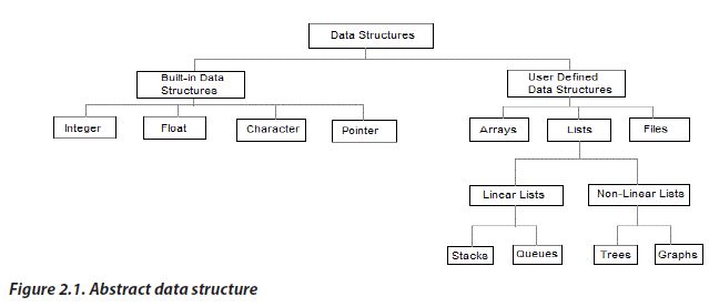 2.1.2. Importance of data structuresThe data structures have the following importance for programming:• Data structures study how data are stored in a computer so that operations
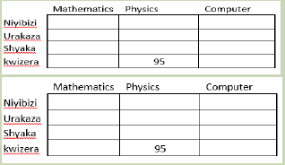 Answer the following questions.1. Suggest a name for the above table?2. How many rows and columns in the above table?3. Identify the location of the value 95 in the above table?Arrays hold a series of data elements, usually of the same size and data type.
 b. Multi-dimensional arrays
 a[i][j] means that it is an element located at the intersection of row i and column j.
 If the table is called marks, marks [1][3]=15; where the row position is 1 and the
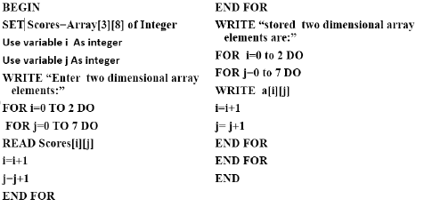 APPLICATION ACTIVITY 2.2.1. Write an algorithm to do the following operations on a two dimensional
 1. Observe and analyze the above figure2. Explain different procedures that you can use to arrange the above books.2.3.1. Definition of Abstract Data type in data structure.Abstract Data structure is a mathematical model of a data structure that specifies the
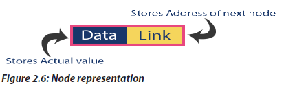 In a single linked list, the address of the first node is always stored in a reference node
 Algorithm in Single Linked ListCreating and read an element in a NODE
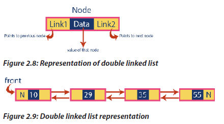 Algorithm in Double Linked ListInserting at Specific location in the list (After a Node)We can use the following steps to insert a new node after a node in the double
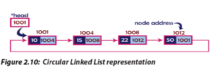 Algorithm in Circular Linked ListInserting at Specific location in the list (After a Node)We can use the following steps to insert a new node after a node in the circular
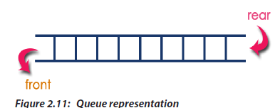 2.5.1 Types of queuesThere exist two types of queues:• Linear queue• Circular queuea. Linear QueueQueue data structure is a linear data structure in which the operationsare performed based on FIFO principle. Queue Operations using Array
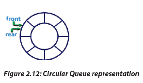 Circular Queue OperationTo implement a circular queue data structure using array, we first create it.• Step 1: Include all the header files which are used in the program and define a
 A Stack is a Last in First out (LIFO) dynamic table or data structure. It has the following
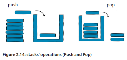 2.6.1 Operations performed on stacksThe different operations performed on stacks are as follows:• Push: adds an element to the stack• Pop: removes an element from the stack• Peek: display at top element of the stackStack Operations using ArrayBefore implementing actual operations, first follow the below steps to create an
 2.7.1 Tree TerminologyIn a tree data structure, we use the following terminology:a. RootIn a tree data structure, the first node is called as Root Node. Every tree must have
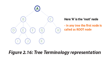 b. EdgeIn a tree data structure, the connecting link between any two nodes is called an Edge.
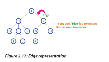 c. ParentIn a tree data structure, the node which is predecessor of any node is called a
 d. ChildIn a tree data structure, the node which is descendant of any node is called a CHILD
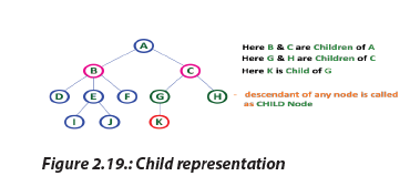 e. Siblings
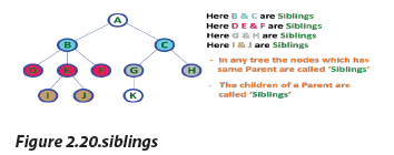 In a tree data structure, the node which does not have a child is called a LEAF Node.
 g. Internal NodsIn a tree data structure, the node which has at least one child is called INTERNAL Node.
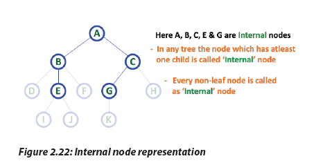 h. Degree
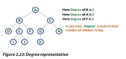 i. LevelIn a tree data structure, the root node is said to be at Level 0 and the children of root
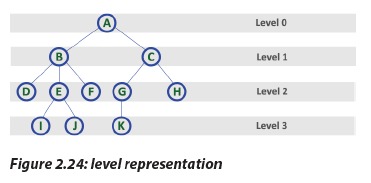 j. HeightIn a tree data structure, the total number of edges from leaf node to a particular
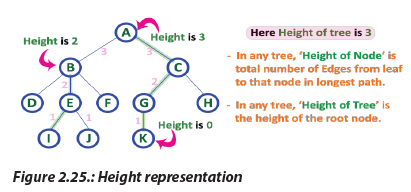 Figure 2.25.: Height representation
 l. PathIn a tree data structure, the sequence of Nodes and Edges from one node to another
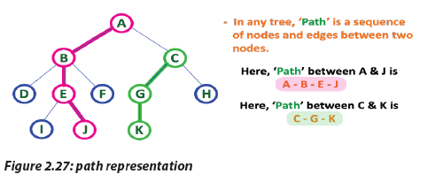 m. Sub TreeIn a tree data structure, each child from a node forms a sub tree recursively. Every
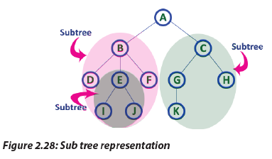 2.7.2 Binary Tree RepresentationsA binary tree data structure is represented using two methods. Those methods are
 In this representation of binary tree, root will contain the location of the root R of T.
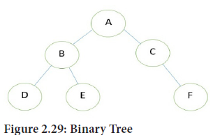 Linked Representation of the Binary Tree
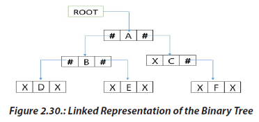 b. Array Representation of Binary Tree
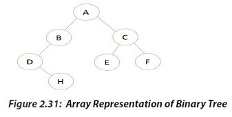 Its sequential representation is as follow:
 2.7.3 Binary Tree TraversalsWhen we wanted to display a binary tree, we need to follow some order in which all
 We start from A, and following in-order traversal, we move to its left subtree B. B is
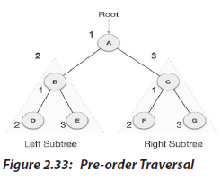 We start from A, and following pre-order traversal, we first visit A itself and then
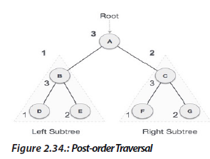 We start from A, and following Post-order traversal, we first visit the left sub tree B. B is also
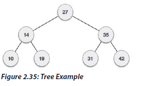 2.7.4. Basic Operations on binary treeA Binary Search Tree (BST) is a tree in which all the nodes follow the below-mentioned