Unit 5 Bivariate statistics and Applications
Key unit competence: Apply bivariate statistical concepts to collect, organise,
analyse, present, and interpret data to draw appropriatedecisions.
Introductory activity
In Kabeza village, after her 9 observations about farming, UMULISA saw
that in every house observed, where there is a cow (X) if there is alsodomestic duck (Y), then she got the following results:
(1,4) , (2,8) , (3,4) , (4,12) , (5,10)
(6,14) , (7,16) , (8,6) , (9,18)
a) Represent this information graphically in (x, y) − coordinates .
b) Find the equation of line joining any two point of the graph and
guess the name of this line.
c) According to your observation from (a), explain in your own
words if there is any relationship between Cows (X) anddomestic duck (Y).
5.1 Introduction to bivariate statistics.
5.1.1. Key concepts of bivariate statistics
Learning Activity 5.1.1
If a businessman wants to make future investments based on how ice cream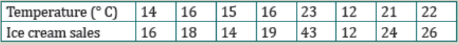
sales relate to the temperature,
i) Which statistical measure and variables will he use?
ii) Which variable depends on the other?
iii) In statistics, how do we call a variable which depends on the other?
iv) Plot the corresponding points (x, y) on a Cartesian plane and describe
the resulting graph. Can you draw a line roughly representing thepoints in your graph?
v) Can you obtain a rule relating x and y ? Explain your answer.
CONTENT SUMMARY
Bivariate data is data that has been collected in two variables, and each data
point in one variable has a corresponding data point in the other value. Bivariate
data is observation on two variables, whilst univariate data is an observation on
only one variable. We normally collect bivariate data to try and investigate the
relationship between the two variable sand then use this relationship to informfuture decisions.
Bivariate statistics deals with the collection, organization, analysis,
interpretation, and drawing of conclusions from bivariate data. Data sets that
contain two variables, such as wage and gender, and consumer price index and
inflation rate data are said to be bivariate. In the case of bivariate or multivariate
data sets we are often interested in whether elements that have high values ofone of the variables also have high values of other variables.
In bivariate statistics, we have independent variable and dependent variable.
Dependent variable refers to variable that depends on the other variable (s).Independent variable refers to variable that affects the other variable (s).
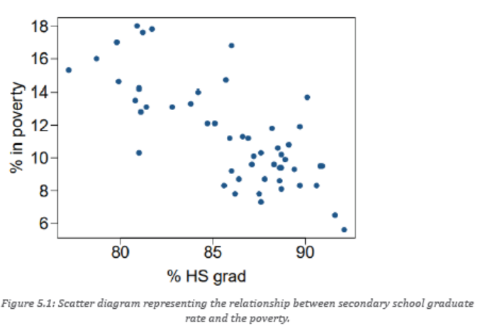
Scatter diagram is the graph that represents the bivariate data in x and y
cartesian plane. The points do not lie on a line or a curve, hence the name. A
scatter graph of bivariate data is a two-dimensional graph with one variable on
one axis, and the other variable on the other axis. We then plot the corresponding
points on the graph. We can then draw a regression line (also known as a line of
best fit), and look at the correlation of the data (which direction the data goes,
and how close to the line of best fit the data points are).For example, the scatter
diagram showing the relationship between secondary school graduate rate andthe % of residents who live below the poverty line.
Examples of bivariate statistics
• Collecting the monthly savings and number of family members’ data
of every family that constitutes your population if you are interested in
finding the relationship between savings and number of family members.
In this case, you will take a small sample of families from across the country
to represent the larger population of Rwanda. You will use this sample to
collect data on family monthly savings and number of family members.
• We can collect data of outside temperature versus ice cream sales, these
would both be examples of bivariate data. If there is a relationship showing
an increase of outside temperature increased ice cream sales, then shops
could use this information to buy more ice cream for hotter spells duringthe summer.
Application activity 5.1.1
1. Using an example, differentiate univariate statistics from bivariate
statistics.
2. Using an example, differentiate dependent variable fromindependent variable.
5.2 Measures of linear relationship between two variables:
covariance, Correlation, regression line and analysis,and spearman’s coefficient of correlation.
5.2.1 Covariance and correlation.
Learning Activity 5.2.1
As students of economics, you might be interested in whether people with
more years of schooling earn higher incomes. Suppose you obtain the data
from one district for the population of all that district households. The data
contain two variables, household income (measured in FRW) and a number
of years of education of the head of each household.
i) Which statistical measure will you use to know whether people with
more years of schooling earn higher incomes.
ii) If you want to know how household income and year of schoolingcovariate, which statistical measure will you consider?
CONTENT SUMMARY
Covariance is a statistical measure that describes the relationship between a
pair of random variables where change in one variable causes change in another
variable. It takes any value between -infinity to + infinity, where the negative
value represents the negative relationship whereas a positive value represents
the positive relationship. It is used for the linear relationship between variables.It gives the direction of relationship between variables.
The covariance of annual household income and schooling years from the
learning activity 5.2.1 is given by
The covariance of variables x and y is a measure of how these two variables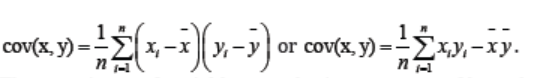
change together. If the greater values of one variable mainly correspond with the
greater values of the other variable, and the same holds for the smaller values,
i.e., the variables tend to show similar behavior, the covariance is positive. In
the opposite case, when the greater values of one variable mainly correspond
to the smaller values of the other, i.e., the variables tend to show opposite
behavior, the covariance is negative. If covariance is zero, the variables are said
to be uncorrelated, meaning that there is no linear relationship between them.Correlation
The Pearson’s coefficient of correlation (or product moment coefficient of
correlation or simply coefficient of correlation), denoted by r , is a measureof the strength of linear relationship between two variables. The coefficient
There are three types of correlation:
• Negative correlation
• Zero correlation
• Positive correlation
If the linear coefficient of correlation takes values closer to -1, the correlation is
strong and negative, and will become stronger the closer r approaches -1.
If the linear coefficient of correlation takes values close to 1, the correlation is
strong and positive, and will become stronger the closer r approaches 1. If the
linear coefficient of correlation takes values close to 0, the correlation is weak.
If r = 1 or r=-1, there is perfect correlation and the line on the scatter plot is
increasing or decreasing respectively. If r = 0, there is no linear correlation.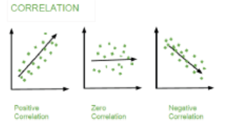
Application activity 5.1.1
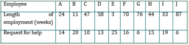
The production manager had ten newly recruited workers under him. For
one week, he kept a record of the number of times that each employee
needed help with a task and make a scatter diagram for the data. Whattype of correlation is there?
5.2.2 Regression line and analysis
Learning Activity 5.2.2
In a village, Emmanuella visited nine families and their farming
activities. For each visited family there were x number of cows,
and y goats. Emmanuella recorded her observations as follows:
(1, 4),(2,8),(3, 4),(4,12),(5,10),(6,14),(7,16),(8,6),(9,18) .
a) Represent Emmanuella’s recorded observations graphically in
cartesian plane.
b) Connect any two points on the graph drawn above to form a
straight line and find equation of that line. How are the positions
of the non-connected points vis-à-vis that line?
c) According to your observation from a., is there any relationship
between the variation of the number of cows and the number of
goats? Explain.CONTENT SUMMARY
Bivariate statistics can help in prediction of a value for one variable if we know
the value of the other. We use the regression line to predict a value of y for any
given value of x and vice versa. The “best” line would make the best predictions:
the observed y-values should stray as little as possible from the line. This straight
line is the regression line from which we can adjust its algebraic expressionsand it is written as y = ax + b .
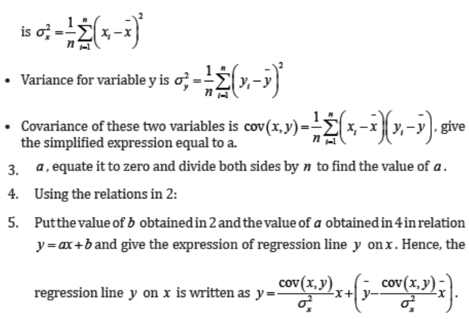
Deriving regression line equation
The regression line y on x has the form y = ax + b . We need the distance from
this line to each point of the given data to be small, so that the sum of the squareof such distances be very small.
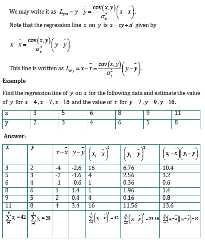
1. Differentiate relation (1) with respect to b . In this case, x, y and a will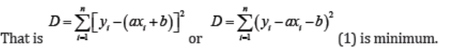
be considered as constants.
2. Equate relation obtained in 1 to zero, divide each side by n and give thevalue of b .
• Take the value of b obtained in 2 and put it in relation obtained in 1.Differentiate the obtained relation with respect to Variance for variable x
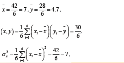
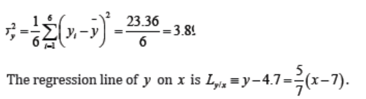
Application activity 5.1.1
Consider the following data:
Find the regression line of y on x and deduce the approximated value of y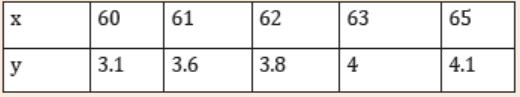
when x=64.
5.2.3 Spearman’s coefficient of correlation
Learning Activity 5.2.2
The death rate data from 1995 to 2000 for developed and underdevelopedcountries are displayed in the table below.
i) Write the death rate for developed countries and the death rate for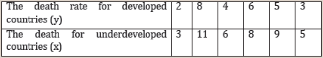
underdeveloped countries in ascending order.
ii) Rank the death rate for developed countries and the death rate for
underdeveloped countries such that the lowest death rate is ranked 1and the highest death rate is ranked 6.
iii) Complete the table below using the information above.
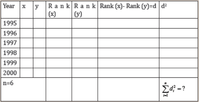
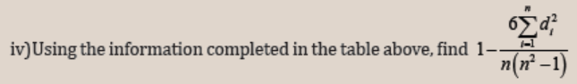
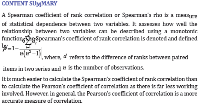
Application activity 5.2.3
Calculate Spearman’s coefficient of rank correlation for the series.
5.2.4 Application of bivariate statistics
Learning Activity 5.2.4
Referring to what you have learnt in this unit, discuss how bivariatestatistics is used in our daily life.
CONTENT SUMMARY
Bivariate statistics can help in prediction of the value for one variable if we know
the value of the other. Bivariate data occur all the time in real-world situations
and we typically use the following methods to analyze the bivariate data:
• Scatter plots
• Correlation Coefficients
• Simple Linear Regression
The following examples show different scenarios where bivariate data appears
in real life.
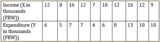
Businesses often collect bivariate data about total money spent on advertising
and total revenue. For example, a business may collect the following data for 12consecutive sales quarters:
This is an example of bivariate data because it contains information on exactly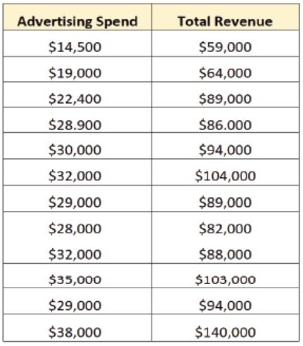
two variables: advertising spend and total revenue. The business may decide to
fit a simple linear regression model to this dataset and find the following fitted
model:
Total Revenue = 14,942.75 + 2.70*(Advertising Spend). This tells the business
that for each additional dollar spent on advertising, total revenue increases by
an average of $2.70.
• Economists often collect bivariate data to understand the relationship
between two socioeconomic variables. For example, an economist may
collect data on the total years of schooling and total annual income amongindividuals in a certain city:
He may then decide to fit the following simple linear regression model:
Annual Income = -45,353 + 7,120*(Years of Schooling). This tells the economist
that for each additional year of schooling, annual income increases by $7,120
on average.
• Biologists often collect bivariate data to understand how two variables are
related among plants or animals. For example, a biologist may collect dataon total rainfall and total number of plants in different regions:
The biologist may then decide to calculate the correlation between the two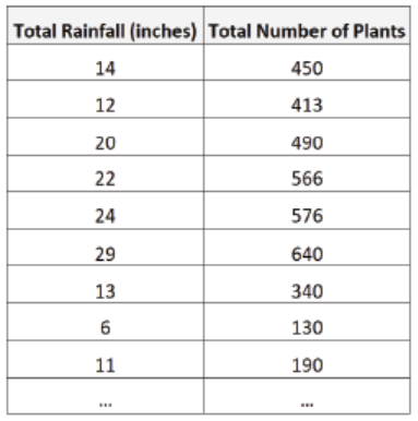
variables and find it to be 0.926. This indicates that there is a strong positive
correlation between the two variables. That is, higher rainfall is closely
associated with an increased number of plants in a region.
• Researchers often collect bivariate data to understand what variables
affect the performance of students. For example, a researcher may collect
data on the number of hours studied per week and the corresponding GPAfor students in a certain class:
She may then create a simple scatter plot to visualize the relationship between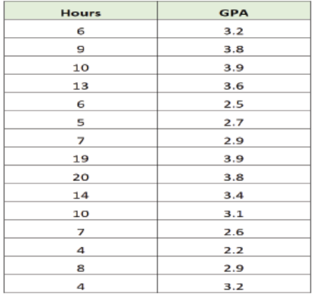
these two variables:
Clearly there is a positive association between the two variables: As the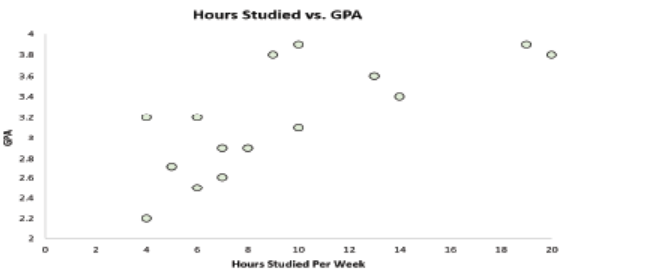
number of hours studied per week increases, the GPA of the student tends toincrease as well.
With the use of bivariate data we can quantify the relationship between
variables related to promotions, advertising, sales, and other variables.
Time series forecasting allows financial analysts to predict future revenue,expenses, new customers, sales, etc. for a variety of companies.
Application activity 5.2.3
A company is to replace its fleet of cars. Eight possible models are
considered and the transport manager is asked to rank them, from 1 to 8,
in order of preference. A saleswoman is asked to use each type of car for
a week and grade them according to their suitability for the job (A-verysuitable to E-unsuitable). The price is also recorded:
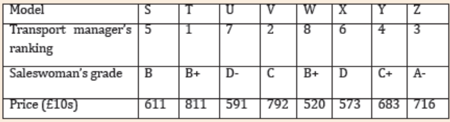
a) Calculate the Spearman’s coefficient of rank correlation between:
i) Price and transport manager’s rankings,
ii) Price and saleswoman’s grades.
b) Based on the result of a, state, giving a reason, whether it would
be necessary to use all the three different methods of assessingthe cars.
c) A new employee is asked to collect further data and to do some
calculations. He produces the following results: The coefficient ofcorrelation between
i) Price and boot capacity is 1.2,
ii) Maximum speed and fuel consumption in miles per gallons is -0.7,
iii) Price and engine capacity is -0.9. For each of his results, say givinga reason, whether you think it is reasonable.
d) Suggest two sets of circumstances where Spearman’s coefficient
of rank correlation would be preferred to the Pearson’s coefficientof correlation as a measure of association.
End of unit assessment 5
1. Table below shows the marks awarded to six students in accountingcompetition:
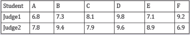
Calculate a coefficient of rank correlation.
2. At the end of a season, a league of eight hockey clubs produced the
following table showing the position of each club in the league andthe average attendance (in hundreds) at home matches.
Calculate Spearman’s coefficient of rank correlation between the position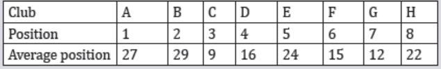
in the league and average attendance. Comment on your results.
3. The following results were obtained from lineups in Accountingand Finance examinations:
Find both equations of regression lines. Also estimate the value of y for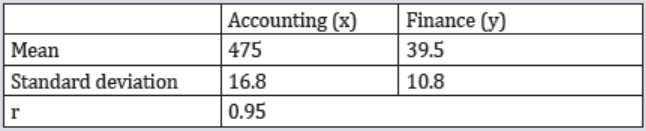
x=30.
4. The following results were obtained from records of age (x) andsystolic blood pressure
of a group of 10 men:
Find both equations of the regression lines. Also estimate the blood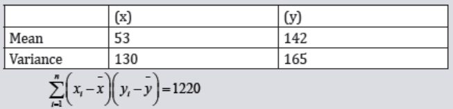
pressure of a man whose age is 45.
REFERENCES
1. Arem, C. (2006). Systems and Matrices. In C. A. DeMeulemeester, Systems
and Matrices (pp. 567-630). Demana: Brooks/Cole Publishing 1993 &Addison-Wesley1994.
2. Kirch, W. (Ed.). (2008). Level of MeasurementLevel of measurement BT
- Encyclopedia of Public Health (pp. 851–852). Springer Netherlands.https://doi.org/10.1007/978-1-4020-5614-7_1971
3. Crossman, Ashley. (2020). Understanding Levels and Scales of
Measurement in Sociology. Retrieved from https://www.thoughtco.
com/levels-of-measurement-3026703
4. Markov. ( 2006). Matrix Algebra and Applications. In Matrix Algebra andApplications (pp. p173-208.).
5. REB, R.E (2020). Mathematics for TTCs Year 2 Social Studies Education.Student’s book.
6. REB, R.E (2020). Mathematics for TTCs Year 3 Social Studies Education.Student’s book
7. REB, R.E (2020). Mathematics for TTCs Year 1 Science MathematicsEducation. Students’ book
8. REB, R.E (2020). Mathematics for TTCs Year 1 Social Studies Education.Student’s book
9. Rossar, M. (1993, 2003). Basic Mathematics For Economists. London andNew York: Taylor & Francis Group.