UNIT 3: CONSUMER BEHAVIOUR

Key unit competence: To be able to analyze the influence of consumer behaviors in allocation of economic resources.
Introductory activity
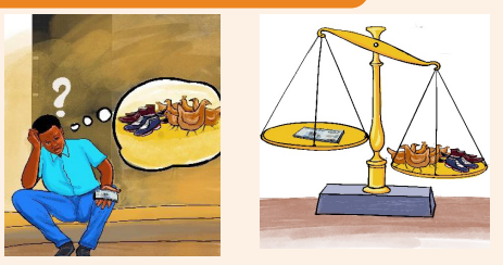
Kalisa has only 20,000FRW (his budget constraint), he must choose how to allocate his funds between buying school shoes and buying hens (the bundle of goods).
If, each pair of school shoes cost 1000 frws and a hen costs 2000 frws, Kalisa can purchase any combination of school shoes and hens that costs no more than 20,000frws.
He could decide to buy only school shoes, or buy only hens, or a combination of both shoes and hens, or he could keep all 20,000FRW in his pocket. Kalisa is able to choose different bundles of goods and services; logically, he chooses those that bring the greatest benefit (or maximizes utility).
Required: In reference to the photographs and case study above;
a) What economic term is given to Kalisa’s act of purchasing school shoes and hens?
b) What is the aim of Kalisa, as he tries to purchase the two items?
c) If Kalisa decided to use all his income to purchase either school shoes or hens, how many units would he purchase?
d) Given alternatives to choose from, why may you buy more of one commodity than the other?
3.1. Meaning of conceptual terms
Learning activity 3.1:
Define the following economic terms:
i) Consumer
ii) Consumer behavior
iii) Utility
iv) Marginal utility
v) Disutility
vi) Total utility
a) A consumer:
Consumer is the final user of goods and services to satisfy his/her wants. i.e. a person or household that buys a final product for use. The main aim of a consumer is utility maximization (satisfy his/her wants) by buying from the cheapest source possible. The consumer demand for a product is based on the utility derived from it. From product point of view, utility refers to the power of a commodity to satisfy consumer wants.
b) Consumer behavior
Consumer behavior refers to the study that analyzes how consumers make decisions about their wants, needs, purchases, or actions related to a product, service, or organization. Understanding consumer behavior is very important in order to analyze potential consumers’ behavior towards a new product or service. It is also very useful for companies to identify opportunities that have not yet been exploited.
The companies that fail to monitor consumer behavior are unable to fill this gap in the market and are left behind. Understanding consumer behavior enables proactive companies to increase their market share by anticipating the shift in consumer choice
c) Utility
Utility is the satisfaction that is derived from consuming a product. Different people have different needs. These needs have to be satisfied. Consumers do not buy commodities for the sake of buying them. They purchase commodities to use them to satisfy their needs.
d) Disutility
Disutility: refers to negative loss of satisfaction derived from consuming more units of a commodity (negative satisfaction).
e) Total utility
Total utility (TU) is the overall satisfaction derived by a consumer from consumption of various units of a good or service, at a certain point or over a period. For instance, if one person takes one cup of tea and another takes two cups, the two may not get the same utility. As one continues to consume more units of a given commodity, he/she reaches maximum satisfaction or saturation point / bliss point/ point of satiety of a consumer. Extra units consumed after this point of satiety cease to provide satisfaction but instead provide dissatisfaction or negative satisfaction. This means that total utility starts declining.
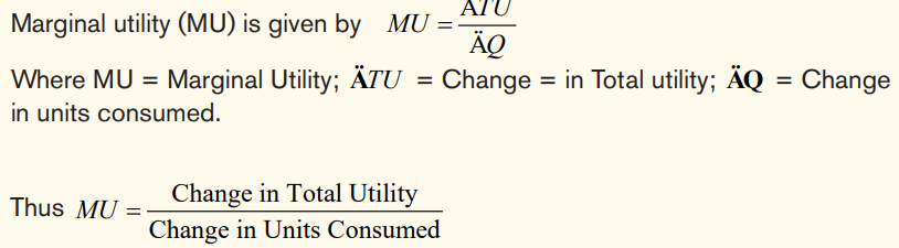
f) Marginal utility
Marginal utility refers to the additional/extra satisfaction received by a consumer on the consumption of an extra unit of a commodity. It implies the addition to the total utility, due to the consumption of one more unit of a good or service. Marginal Utility is also known as “marginal satiety”. As more units of a commodity are consumed, total utility increases because each new unit consumed adds to the total. This means that as one adds more units of a commodity, there is extra or additional satisfaction to him/her thus Marginal utility (MU).
Application activity 3.1
Make short notes and present to the class about the scenarios of what happen under the following economic terms:
a) Utility (b) Total utility (c) Marginal utility (d) Disutility
3.2. Relationship between Total Utility and Marginal Utility
Learning activity 3.2:
Given that the relationship between TU and MU is such that:
• When TU is increasing, MU is decreasing.
• When TU is at the maximum, MU is zero.
• When TU is decreasing, MU is in negative. (Disutility)
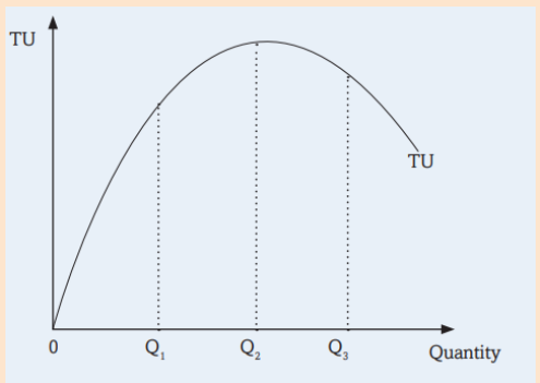
State the nature of MU at:
(a) Q1
(b) Q2
(c) Q3
Total Utility can be expressed as: TUn = Ux + Uy + Uz or TU = MU
Where TU = Total Utility n = Number of commodities
Ux , Uy , Uz = Total respective utilities of consumption of goods
MU = Marginal Utility.
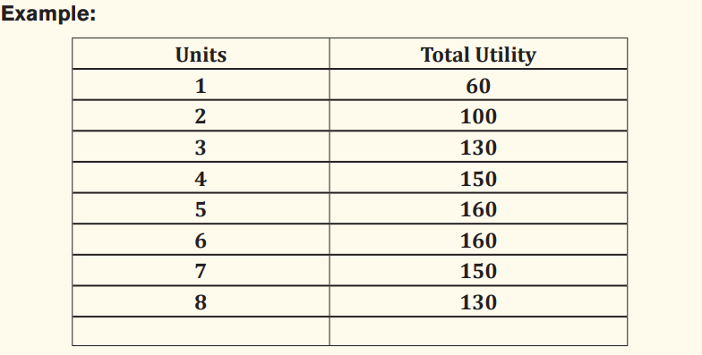
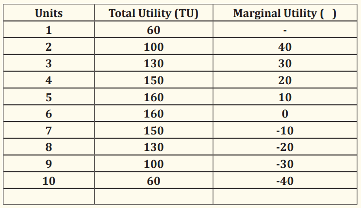
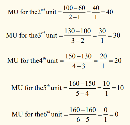
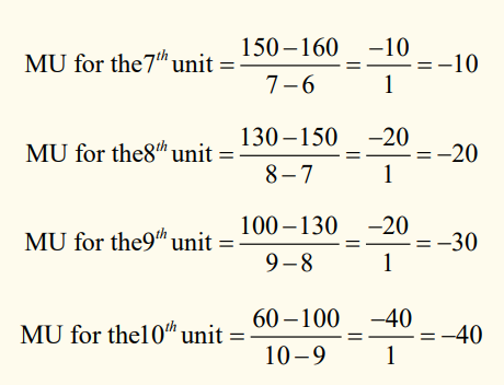
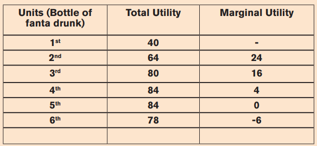
From the above table, we plot total utility as below:
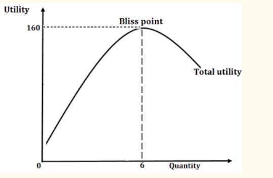
From above illustration, total utility increases up to 6th unit. At this point, the consumer has reached his or her point of saturation (maximum point of satisfaction). As consumption goes beyond 6th unit, total utility starts to reduce. The consumer gains no more utility for consuming a given product. Consumption of the commodity beyond total satisfaction (point of saturation) leads to disutility or negative satisfaction.
Marginal Utility Curve:
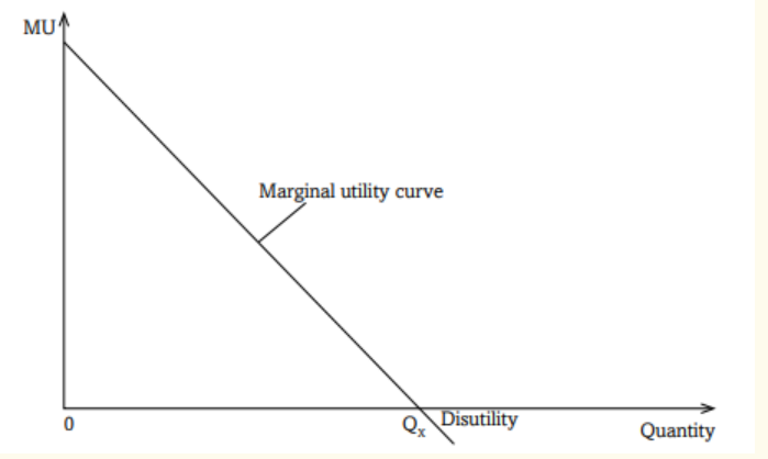
If more and more units of a good are consumed, the additional utility from each additional unit consumed continues to decrease and even becomes negative. This means that marginal utility is temporarily negative.
Suppose that you are hungry and buy food for dinner. Let’s also say that a plate of food costs 2500frw. If you are so hungry that you would pay 3,000frw for the plate of food, the food is said to provide 3,000frw worth of benefit. In other words, you’re willing to pay 3000frw to get the satisfaction out of the plate of food no matter what it actually costs.
Total utility is just the concept of utility applied to more than one good. If consuming a good brings you a certain utility, consuming more goods of the same good will get you more, less, or the same amount.
E.g.: Assume that you plan to eat two plates of food. However, after eating the first plate, you’re not quite as hungry as you were before. Now you only pay a lower price, e.g. 2000frw for the additional utility of the second plate. It’s not worth that much to you now that you’re a little fed up. This means that the two plates of food together provide 2000frw (2nd plate of food) + 3000 frw (first plate of food) = 5000frw of total utility. A consumer would ultimately not buy the extra plate of food because their marginal utility (2000frw) is less than their marginal cost (2500frw). Basically, you lose utility in this transaction, so it’s not in your favor.
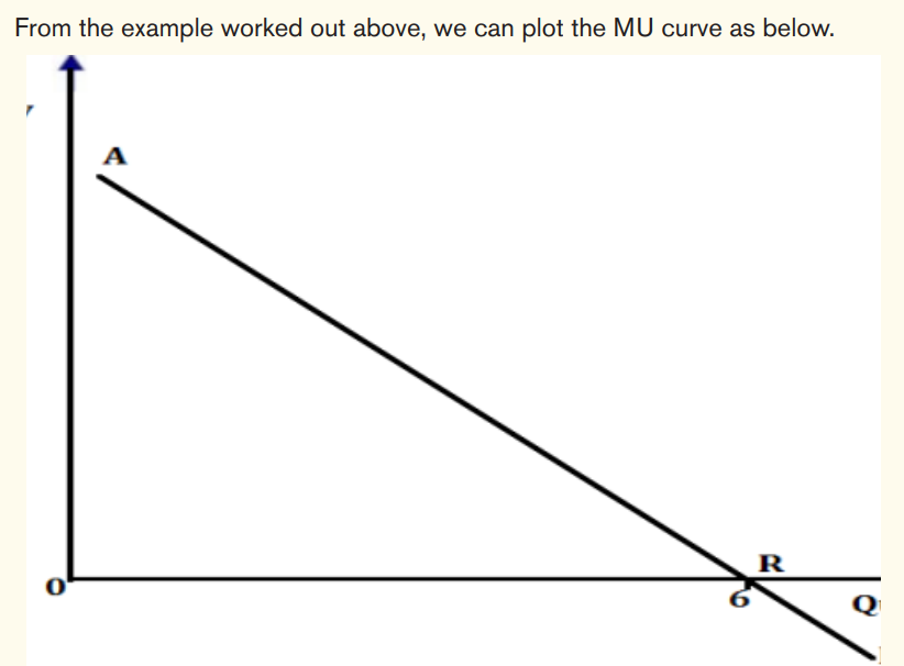
From point A to point R, MU is still positive. At point R, MU is zero (0) and after that point, MU becomes negative (disutility). If the additional consumption of a commodity generates less satisfaction than the previous one, the consumer is willing to pay less for any additional unit to be consumed. This makes the consumers demand decrease as he/she consumes more units of a commodity, which explains the shape of the marginal utility curve.
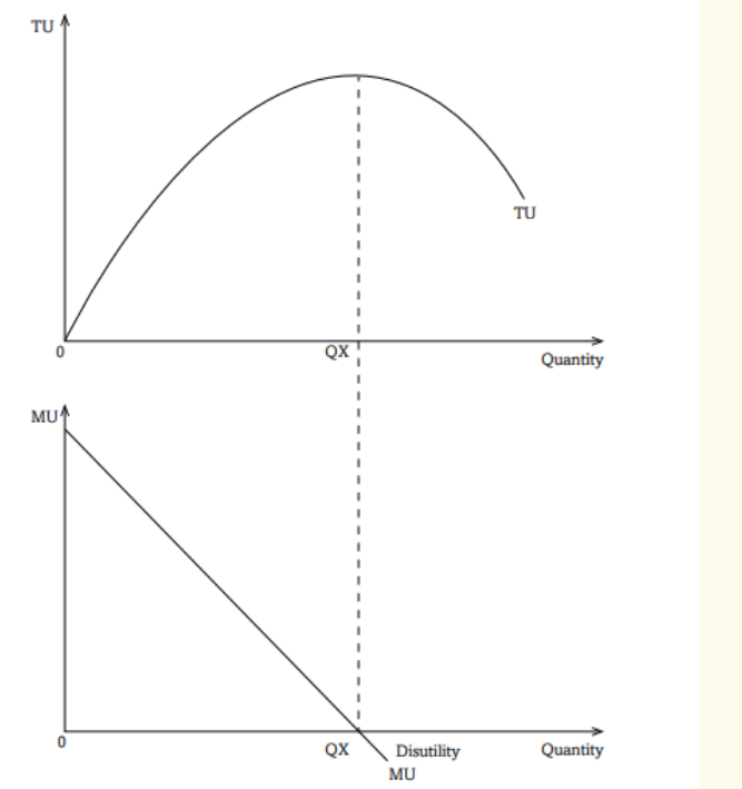
Note the following relationship between Total Utility and Marginal Utility:
– When TU is increasing, MU is decreasing.
– When TU is at maximum, MU is zero.
– When TU is decreasing, MU is negative (disutility).
Illustration of relationship between TU & MU:
MU, from the 1st unit isn’t known because the TU before the 1st unit isn’t indicated. After the 1st unit TU is increases but at a decreasing rate. After the 6th unit, TU declines because MU becomes negative due to disutility or negative satisfaction (utility) which sets in.
For example, one may start vomiting after the 6th unit, a situation that reduces TU he/she had gained. The 1st units of a commodity give a higher satisfaction than the subsequent units. This is because the need that the commodity covers is gradually satisfied. The quantity consumed and MU vary inversely.
This relationship can be illustrated as below:
Disutility is the negative or dissatisfaction that is derived from the over consumption of a good or service. For instance, if you consume too much soda to the extent of vomiting you will have gone into dissatisfaction.
Application activity 3.2
The table below shows Kalisa’s utility got from consuming eight bottle of soda of the same brand
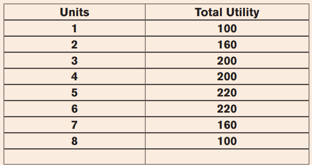
Use the above information:
a) To calculate the marginal utility
b) To plot total utility and marginal utility
3.3. The law of diminishing marginal utility, its assumptions and application
Learning activity 3.3:
Use the information on the table below to answer the questions that follow assuming that a thirsty consumer took successive bottles of soda until his/ her satisfaction:
Imagine you were this consumer,
a) Which bottle took less time to finish and why?
b) Which bottle was enjoyed most?
c) Which bottle do you think was highly or less paid for and why?
The law of diminishing marginal utility states that: “As a consumer consumes more and more units of a specific commodity, the utility from the successive units goes on diminishing”
Assumptions of the law of Diminishing Marginal Utility.
i) The consumer is rational and strives for utility maximization.
ii) The goods are taken in reasonable and suitable units. If the units are too small, then the MU can increase to a few units instead of falling.
iii) Constant taste of a consumer; That is, the law applies when a consumer’s tastes do not change. E.g. if a consumer develops a taste for wine, the additional units of wine may increase the MU.
iv) The consumption must be continuous, without abnormal and prolonged intervals between the consumption of different units. For example, if you eat one plate of food in the morning and the second in the afternoon, the MU of the second plate of food may increase
Let us explain the law of Diminishing Marginal Utility by using an example:
Suppose someone is very thirsty. He/she goes to the market and buys a glass of water. The glass of water gives him great pleasure or we say the first glass of water is of great utility to him/her. If he/she then takes a second glass of water, the utility is less than that of the first. This is because the edge of his/her thirst has been greatly reduced. If he/she drinks a third glass of water, the utility the third glass will be less than that of the second, and so on.
The utility continues to decrease with the consumption of each successive glass of water until it falls to zero. This is the saturation point. It is the position of consumer’s equilibrium or maximum satisfaction. Continuing to force the consumer to drink a glass of water results in disutility, thereby reducing total utility. The marginal utility will become negative.
A rational consumer will stop taking water at the point where marginal utility becomes zero, even if the good is free. In short, the more we have of something, ceteris paribus, the less we want more of it, or more precisely. The more a consumer receives of a given product in a given period of time, the less eager he is to obtain more units of that product, or we can say that additional units provide less additional satisfaction when more units of a good are consumed than previous units.
Relationship between MU and demand curves.
This law explains why the demand curve slopes from left to right. When a consumer gets high marginal utility from a unit of a commodity, he is willing to pay a high price for it. If the amount consumed increases and marginal utility decreases, the consumer is willing to pay a lower price.
The demand curve corresponds only to the positive part of the MU curve. The demand curve does not intersect the x-axis because we cannot have negative price even though we have negative MU. This can be illustrated as follows.
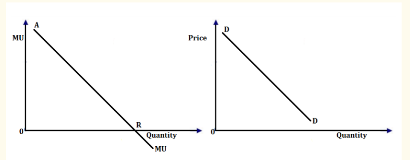
When MU decreases, the consumer is willing to pay less for the goods. This indicates that the price of a commodity depends on the MU. The higher the MU, the higher the price and vice versa. Because MU is high, the price is high, but the demand is lower. When MU falls, one is willing to pay less for the commodity, hence demand is high
Application activity 3.3
Observe and analyze the graph below:
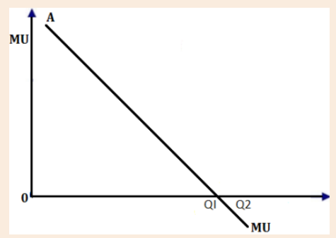
a) Which point shows total utility when it is at maximum and support your answer.
b) Explain where the total utility would be at point Q2.
3.4. The budget line
Use the formula below to answer the following questions. Px × Qx + P y × Q y = Y (price of x times its quantity plus price of y times its quantity = income).
Given that the price of commodity X is 1,000Frw per unit while commodity Y costs 500 Frw per unit. John has a fixed income of 20,000Frw, which he wants to spend on the two commodities X and Y.
a) Find how many units of each commodity he will purchase if:
i) He spends 10,000Frw on each commodity.
ii) He spends 12,000Frw on commodity X.
iii) (iii) He spends 15,000 Frw on commodity X.
iv) He spends all his income on commodity X.
v) He spends all his income on commodity Y.
b) Illustrate your findings on a curve.
3.4.1. Meaning, assumption and budget constraint
Meaning of budget line
The quantity that the consumers buy to consume depends on the level of their incomes and the price of the commodities. A budget line is a line that shows various combinations of two commodities that a consumer can purchase using his or her fixed income.
Assumptions of budget line
– Only two commodities can be purchased.
– The price of the items should be given.
– The income to be spent should be given and fixed.
– All income set should be spent.
– All other factors that can influence this analysis should be kept constant throughout the entire analysis.
Budget constraint
This refers to the amount within you spending limit, that is, you cannot spend more money than what you have.
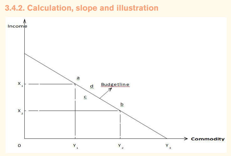
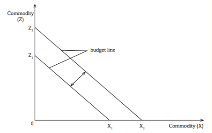
Consider the following graph:
Using the fixed income, the consumer can purchase Y1 units of commodity Y and X1 units of commodity X (combination Y1 X1, point a). The consumer can also purchase Y2 units of commodity Y and X2 units of commodity X (combination Y2 X2, point b) and all the income is used up.
All combinations that lie along the budget line (such as points a and b) show what can be purchased when the consumer’s income is used up.
Points below the budget line (such as point c) show that some income will not be used. Points outside the budget line such as point d, are unachievable with the same level of income.
E.g.: If the income is fixed at 10, 000Frw and the price of sugar and rice is 1, 000Frw per kilogram and 2,000Frw per kilogram respectively, then the consumer can buy 4 kg of sugar and 3 kg of rice and all the income is consumed. Alternatively, with the same income, the consumer can buy 10 kg of sugar alone or 5 kg of rice alone. The following budget line can be derived from these figures.
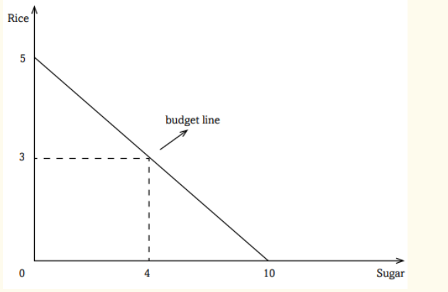
A change in consumer income at constant prices shifts the position of the budget line. An increase in consumer income shifts the budget line to the right, while a decrease in consumer income shifts the budget line to the left. A change in the price of the two goods, given constant consumer income, also shifts the position of the budget line. An increase in the price of the two commodities shifts the budget line to the left, while a decrease in the price of the two commodities shifts the budget line to the right.
• Extension or contraction in the budget Line
A change in price of one commodity shifts the budget line on one side. This is the same when the increase in income is used on one commodity.
A shift in the budget line on one side
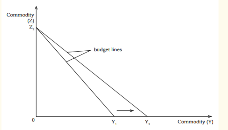
A decrease in the price of commodity Y means that with the same income, the consumer can now buy more of commodity of Y and the budget line shifts to the right on the side of commodity Y from Y1 to Y2 .
The budget line equation
The budget line equation is a mathematical expression that explains the mode of combining quantities of two items using the fixed income-budget constraint.
Let us use an example of Irish potatoes and sweet potatoes to develop the idea. Take y for Irish potatoes and x for sweet potatoes, B for budget constraint price of Irish potatoes 100frw and price of sweet potatoes 50frw. From these, the mathematical arrangement relating the budget constraint, the prices of the two items and their quantity purchased is as follows:
Where:
• B is the budget constraint, let us take 1,000FRW
• X is the quantity of item 1, let us say Irish potatoes.
• is the price of X per unit,
• y is the quantity of item 2, let us say sweet potatoes
• Py is the price of Y per unit.
Given the above data, the budget line is given as: and taking X and Y as variables. The expression is a clear mathematical model called the budget line equation.
This model can be used to find the quantity of X (Irish potatoes) given Y (sweet potatoes), or to find the quantity of Y (sweet potatoes) given X (Irish potatoes).
Let’s use our example to determine the quantity of Irish potatoes (X) that would be purchased if a consumer chose to buy 6 Kgs of sweet potatoes (Y) under the budget line equation
Answer: Given the equation where, X= Irish potatoes and Y= Sweet potatoes If Y=6, Y is substituted in the equation 1000=100X +50Y and we solve for X.
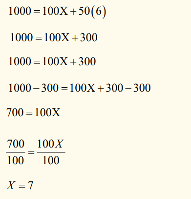
Using the budget line equation model, a consumer will buy only 7Kgs of Irish potatoes when he had chosen to buy 6Kgs of sweet potatoes
• That model would help also to know the direct relationship between the quantities of two items in question. With it, we make one of the items the subject of the formula
Application activity 3.4
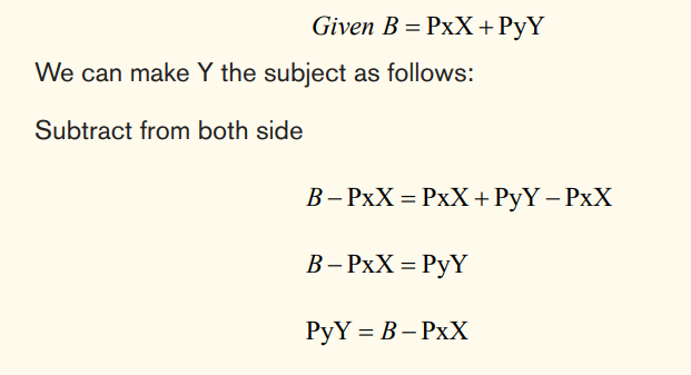
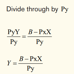
Given the model B = + PxX PyY ,make Y the subject
3.5. Indifference curves
Learning activity 3.5:
Carry out research from the internet and library books, on the:
a) Meaning of the Indifference curve
b) Features of indifference curves.
c) Illustrate your findings on a graph
3.5.1. Meaning and assumptions
Meaning of the Indifference curve
An indifference curve is a curve that shows various combinations of two commodities that give the consumer equal satisfaction. The consumption of any combination of the two commodities that lie along the curve gives the same units of utility.
Assumptions of the Indifference curves
The indifference curves analysis is based upon some assumptions which determine its strength, applicability and shortcomings. The following are various assumptions of indifference curves:
– Rationality: The consumer is assumed to behave in rational manner, that is, his/her main aim is to maximize his/her total utility given his income and market price. He/She also assumed to have full knowledge of market conditions. Furthermore ,he is consistent in his/her choice, that is, if in one situation he/she chooses combination A rather than combination B, he/she will not choose B in preference to A in other situation
– Non satiety: This assumption implies that the consumer has not reached the point of saturation in the consumption of any commodity. Thus, he always prefers to have more of both commodities. He always ties tries to move to a higher indifference curve to get higher and higher satisfaction.
– Two commodities: It is assumed that a consumer has a fixed amount of money whole of which is to be spent on two goods, given constant prices of both goods. This is very restrictive assumption, because, in reality the consumer deals with a large number of commodities. This restrictive assumption is made to facilitate graphic representation of indifference curves.
– Transitivity: Preferences or indifference of a consumer are transitive. Assume there three combinations of two goods A, B and C. If the consumer is indifferent between A and B and also between B and C, it then assumed that he will be indifferent between A and C too. This implies that consumer’s tastes are quite consistent.
– Diminishing of Marginal Rate of Substitution: It is assumed that both the commodities X and Y obey the law of diminishing marginal utility. This law implies, as more and more units of X are substituted for Y, a consumer will be ready to sacrifice less and less units of Y for each additional unit of X. Similarly, a consumer will be ready to give up less and less units of commodity X for each additional unit of commodity Y.
– Positive marginal utilities: The commodities are considered good and have positive marginal utilities. This implies that given any combination of two commodities, increase in quantity of one commodity increases the total satisfaction and vice-versa. Therefore, in order to keep the total utility at the same level, the quantity of one commodity should be increased for every reduction in quantity of other commodity.
– Divisibility: The commodities are assumed to be divisible. This means that quantities of commodities can be increased (or decreased) in minute amounts and the corresponding changes in total satisfaction can also be very small. This assumption makes an indifference curve continuous without curves or breaks.
– Ordinal utility: Utility can be measured only in ordinal terms and not cardinal ones. In other words, consumer cannot measure precisely utility or satisfaction in absolute units. He can conveniently arrange various combinations of two or more commodities in ascending or descending order of preference.
Between any two combinations, he is only able to tell that utility from one combination is more than, equal to, or less than the utility from the other combination. He is not in a position to tell the amount of difference in the utility from any two combinations.
3.5.2. Characteristics and Illustration of indifference curves
Indifference curves have the following characteristics:
– Indifference curves are convex to the origin.
– Indifference curves are parallel to each other for example two indifference curves cannot meet (they cannot intersect each other).
– The indifference curves are negatively sloped
– Indifference curves do not touch the X or Y-axis except when the two commodities X and Z are complete substitutes, that is to say, Indifference curves do not touch the horizontal or vertical axes
– Higher indifference curve represents higher level of satisfaction.
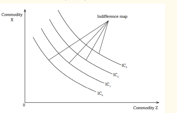
Many indifference curves on the same graph make up an indifference map.
All combinations along the indifference curve give the same satisfaction.
Consider the following indifference curve:
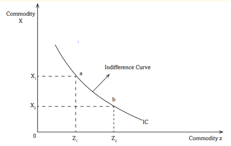
At point a, the consumer takes Z1 units of commodity Z and X1 units of commodity X (combination Z1 X1).
At point b, the consumer takes Z2 units of commodity Z and X2 units of commodity X (combination Z2 X2). In this case, the utility gained at point a is equal to what is gained at point b.
Increase or decrease in satisfaction means that the consumer has increased or decreased consumption of both commodities. This will lead to a shift in the indifference curve. Increase in satisfaction shifts the indifference curve to the right. Decrease in satisfaction shifts the indifference curve to the left. Drawing many indifference curves on one graph gives an indifference map.
Application activity 3.5
Explain the situation which can lead the indifference curve to shift to the right or to the left. Use the graphical representation to demonstrate that shift.
3.6. Consumer equilibrium
Learning activity 3.6:
Conduct a research on:
a) The meaning of consumer equilibrium.
b) How to determine consumer equilibrium using both the indifference curve approach and the marginal utility approach.
3.6.1. Meaning of consumer’s equilibrium, equation and illustration
The consumer strives for maximum satisfaction at the lowest possible cost. The consumer must ensure that he uses less of the disposable income but enjoys it to the maximum.
Consumer equilibrium occurs when the consumer gets maximum equal satisfaction from each unit of his or her income spent on consumption.
This can be explained by two approaches:
a) The utility approach.
b) The indifference curve approach.
3.6.2. Equilibrium using utility and indifference curve approaches
The marginal utility approach explains consumer behavior under the assumption that the consumer consumes only one good while the indifference curve approach assumes two commodities.
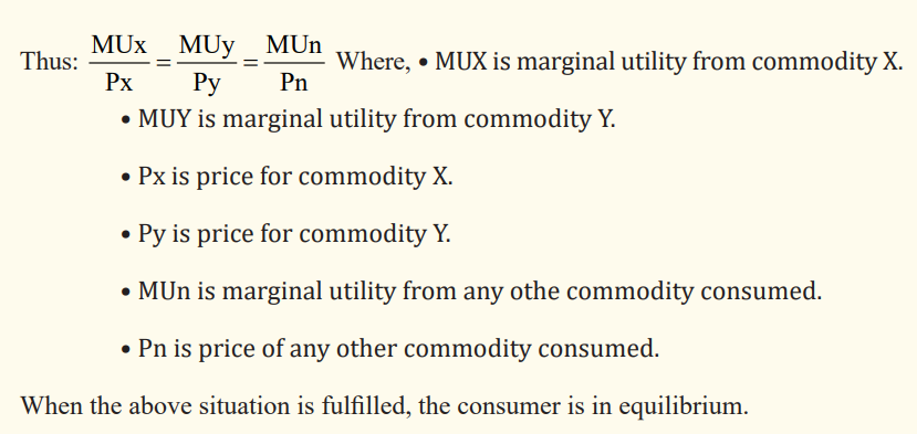
Consumer’s Equilibrium using utility approach
In this approach, the consumer is in equilibrium when the marginal utility derived from spending a unit of his or her income on a unit of commodity X is equal to the marginal utility got from spending his income on commodity Y.
Consumer’s Equilibrium using indifference curve approaches
With this approach, consumer equilibrium occurs at a point where the indifference curve touches the budget line. Consumer equilibrium is reached when the budget line is tangent to the indifference curve.
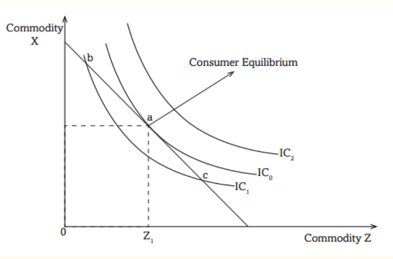
Points a, b, and c lie on the budget line. This implies that the consumer’s income is sufficient to purchase any combination of the two commodities at any of the points.
Indifference curve IC1 is lowest and therefore all points lying on it give
the lowest utility, i.e. point’s b and c are within the consumer’s budget
line but give the lowest satisfaction.
– Point a lies along the highest indifference curve that is within the consumer’s budget line, and therefore provides maximum satisfaction that is affordable for the consumer.
– At point a, where the indifference curve IC0 is tangent to the budget line, the consumer is in equilibrium.
– The indifference curve IC2 is higher but it is outside the budget line. This implies that consumers’ incomes are insufficient to afford a combination along this curve.
Application activity 3.6
1. Explain the consumer’s equilibrium using the following approaches:
a) Utility
b) Indifference curve
3.7. Consumer surplus, producer surplus and social surplus
Learning activity 3.7:
When you visit a market place, you find sellers and buyers negotiating about prices.
(a) In relation to your knowledge of utility, discuss why the buyer negotiates for a lower price.
(b) Using the formula given, calculate the consumer surplus.
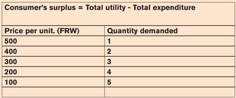
(c) Using 100 as market price find the consumer surplus.
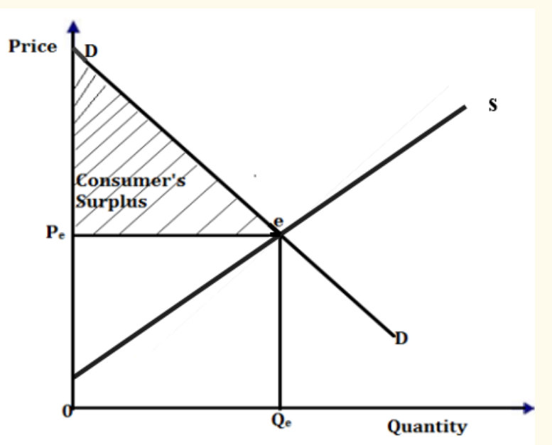
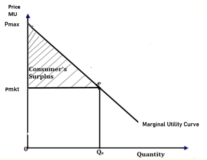
3.7.1. Consumer surplus Consumer surplus is defined as the difference between the total amount that consumers are willing and able to pay for a commodity and the total amount that they actually pay (i.e. the market price).
Consumer surplus is presented by the area under the demand curve and above the price. Consumer surplus is a measure of the welfare that people gain from consuming goods and services. For example, the consumer is willing to pay 1000FRW but the market price is 750FRW, therefore, consumer’s surplus is 200Frw. i.e.: 1000-750 = 250.
As MU diminishes, the consumer is willing to pay less for the successive units of the commodity. Thus, MU diminishes as the consumer’s surplus also diminishes. Consumer surplus always increases as the price of a good falls and decreases as the price of a good rises.
Consumer’s surplus = Price consumer is willing to pay – market price.
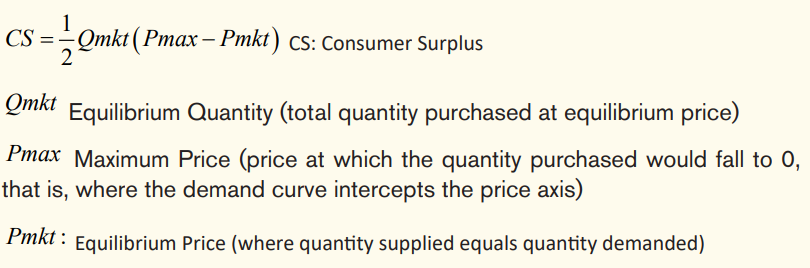
If the demand curve is a straight line, the consumer surplus is the area between the demand curve and equilibrium price. Therefore the consumer surplus is
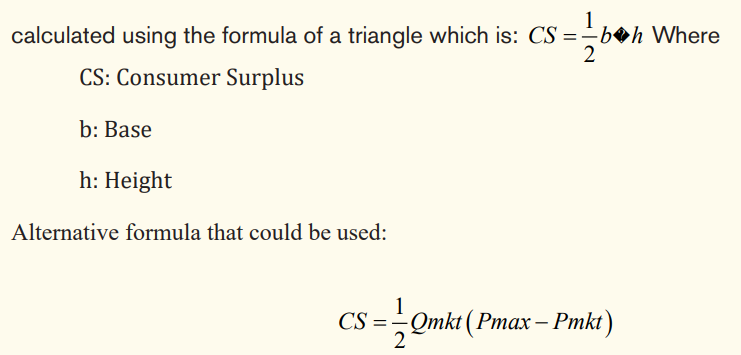
Where
CS: Consumer Surplus
Qmkt: Equilibrium Quantity (total quantity purchased at equilibrium price)
Pmax: Maximum Price (price at which the quantity purchased would fall to 0, that is, where the demand curve intercepts the price axis)
Pmkt: Equilibrium Price (where quantity supplied equals quantity demanded)
By illustration, the consumer’s surplus is the area below the demand curve and above the equilibrium price as seen below
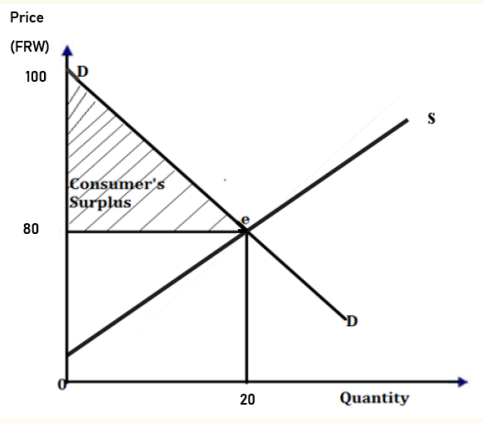
e.g.: Kayiranga is willing and ready to pay 200frw for one mangoes. When he reached the market he found 20 mangoes for 80Frw per one mangoes.
Required:
a) Calculate Kayiranga’s consumer surplus.
b) Use the demand and supply curve to derive Kayiranga’s consumer surplus
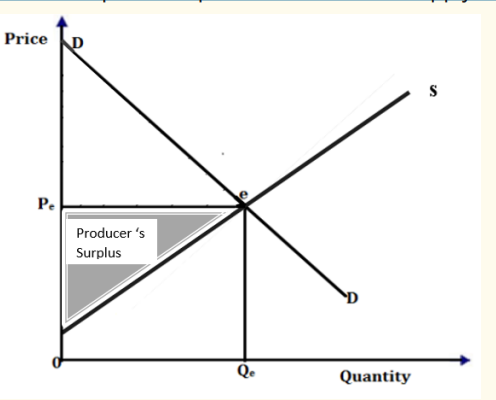
3.7.2. Producer surplus
Producer surplus refers to the difference between the price that the producer is ready and willing to accept for his or her commodity and what he or she actually receives.
The producer usually has a particular price at which he is ready to offer his product for sale. The producer usually has a particular price at which he/she is ready to offer his/her product for sale (reserve price).
Producer surplus is a measure of producer welfare. It is measured as the difference between what producers are willing and able to supply a good for and the price they actually receive.
It is the area below the equilibrium price and above the supply curve.
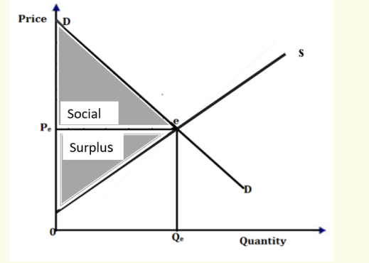
3.7.3. Social surplus
Social surplus is the total sum of the consumer surplus and producer surplus combined.
This can be illustrated as below:
3.7.4. Relationship between consumer surplus, utility and price
Utility is the benefit or satisfaction a consumer gets from using a good or a service. Price and utility are intertwined. If a seller of juice sells it at 400Frw. A consumer will buy it if he expects to get 400Frw worth of utility from the consumption of juice. However, this depends on how thirsty the consumer is at the moment and how much he likes juice.
The price of juice to be paid by the consumer depends on the satisfaction worth the price. In relation to consumer surplus, a consumer pays 400Frw for juice if he thinks the juice provides utility worth 400Frw. Consumers who think juice provides satisfaction more than 400Frw will be willing to pay more, that is to say, 500Frw or even more 600Frw.
Consumer surplus occurs when the price consumers pay for a product or service is less than the price they are willing to pay. It is a measure of the additional benefit consumers receive by paying for something less than they were willing to pay.
A price increase decreases consumer surplus, while a price decrease increases consumer surplus. Marginal utility explains the price a consumer is willing to pay for units of the good purchased, as more goods are purchased, marginal utility falls.
Application activity 3.7
1. Construct the relationship between consumer surplus and the producer surplus
2. Rukundo is a food processing plant owner, he is willing to sell 1litre of yoghurt at 500Frw but the market price is 600Frw. Kwizera who is a consumer is willing and ready to buy 10litres of yoghurts at 800Frw
Determine the:
a) Consumer surplus
b) Producers and the social surplus
Skills Lab 3
Consider your business club as the suppliers of the products of your business club and consider the students as the consumers. In teams, discuss under what circumstances may consumers’ surplus or producers’ surplus occur. Share your findings with the entire class and provide advises to your club (producer) on what to do in case consumer’s wish to pay below market price?
End of unit assessment
3. Given that the price of meat is 2,000 FRW per kg and that of sugar is 2,500 FRW per kg. The income of the consumer is fixed at 50,000Frw. Derive a budget line for this consumer
4. Differentiate between Budget line and Budget constraint
5. Differentiate utility from disutility