Unit 4: E COMMERCE,SOCIAL,MEDIA AND ONLINE SERVICES D ONLINE
Key Unit competence: To be able to request for online services and access social media
4.0 INTRODUCTORY ACTIVITY
Holly City Technology Ltd manager needs to buy computer spare parts products from outside of Rwanda.
The manager doesn’t have time to go out of the country and he decided to search on the Internet the websites which sell computer spare parts.
a. Discuss ways the manager can use to communicate with the supplier to obtain the price of the goods
b. Discuss the type of business conducted via the Internet
c. Give social media platforms used for daily communication
Discuss the way that can be used for payment4.1. E commerce
ACTIVITY 4.1
1. Kamikazi wants to buy a Psychology book. She visited many libraries in the country but she could not find the title she wanted. She decided to search for the book using google.com. Finally, she realized that the book is available online on amazon. com and the price is at 15 $.
a. Discuss the process Kamikazi will go through in order to buy that book and have it delivered to her
b. Brainstorm the other local and global online platforms that can be used to buy goods and services
2. What do you understand by Customer to Business relationship?
4.1.1. Understanding e commerce
a. History
E-Commerce or Electronic Commerce also known as e-Business, Is the buying and selling of goods, products, or services over the internet using electronic means of payment like credit cards. This commerce provides to buying parties physical goods but also electronic materials (goods) where possible.
The history of ecommerce dates back to the invention of the very old notion of “sell and buy”, electricity, cables, computers, modems, and the Internet. Ecommerce became possible in 1991 when the Internet was opened for commercial use
At first, the term ecommerce meant the process of execution of commercial transactions electronically with the help of the leading technologies such as Electronic Data Interchange (EDI) and Electronic Funds Transfer (EFT) which gave an opportunity for users to exchange business information and do electronic transactions. The ability to use these technologies appeared in the late 1970s and allowed business companies and organizations to send commercial documentation electronically.
b. Some Ecommerce platforms
With ecommerce the buying and selling parties don’t need to meet at the same location, the buyer does not go to the store but there is an electronic platform that is used as a market where the buyer and the seller meet. An example of such a platform is amazon.com.
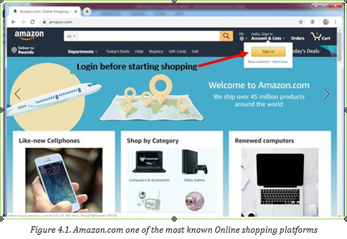
To buy goods on amazon.com or any other online chopping platform (ecommerce website), the buyer must have an Amazon account, must log in using that account, choose among the list of provided goods, choose location where the goods are to be delivered and pay using acceptable payment means like Credit cards.
As of November 2019, the online shopping platforms available in Rwanda are among others food.jumia.rw and kikuu.com. Through this platforms one can buy food (jumia food) or clothes (kikuu.com).
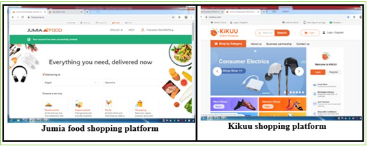
Figure 4. 2. Main interfaces of the shopping platforms in Rwanda (food.jumia.rw and rw.kikuu.com)
a. Buying on an e-commerce platform case of kikuu.com
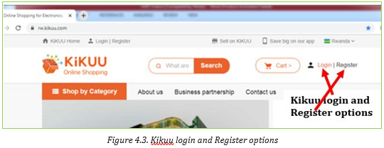
As stated earlier kikuu.com is one of the platforms available in Rwanda with which one can buy available goods and have them delivered to his/her preferred location in Kigali. To buy with Kikuu, as it is a principle for other e-commerce the buyer has to have an account. To create that account go through these steps:
1. In the address bar write kikuu.com and once the platform loads click on Register to create a login account. Fill in the provided form the requested details. Or
2. If the user account is already created login
1. Once the login is successful choose goods to buy.
For most platforms goods have pictures and accompanying image and for selecting the goods just click on its image. Select the goods specifications carefully so as to get what is wanted. In the case of the shoes chosen like in the image below the customer has to choose the shoe’s color and the size.
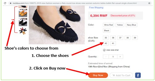
Figure 4. 4. Screen to choose shoe specifications
1. Pay the amount due by using the preferred payment method
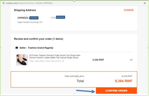
Figure 4. 5. Shipping address and confirm order Window
In the next two screens choose the payment method and click on PAY <Amount>. In the other screen as MTN Money has been chosen as payment method fill the account and click PAY <Amount>
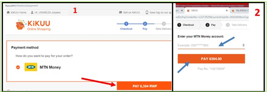
Figure 4. 6. Screens for choosing the payment methods and paying
a. Advantages and disadvantages of e commerce
There is no good thing without a bad side. Ecommerce presents to its users many advantages but has also disadvantages.
a. Advantages of E-commerce
• Does not require physical displacement of the buyer hence saving money and time
• Products and services are easy to find on the platform rather than moving
in so many stores, warehouses or supermarkets
• Transactions can be done all the time of the day and the week (24/7).
• No geographical limitations translates as a bigger customer reach.
• Higher quality of services and lower operational costs.
b. Disadvantages of E-commerce
• No guarantee of product quality as the product is not physically viewed
• Customer loyalty becomes a bigger issue as there is a minimal direct customer-seller interaction.
• Anyone can start an online business, which sometimes leads to scam and phishing sites.
• Hackers target web shops which may lead to disruption of service.
4.1.1. E-commerce models
Electronic commerce can be classified into four main categories. The basis for this simple classification is the parties that are involved in the transactions. The four basic electronic commerce models are:
a. Business to Business
In a business to business model companies are doing business with each other. The final consumer is not involved. So the Online transactions only involve the manufacturers, wholesalers and retailers, etc.
b. Business to Consumer
Here the company will sell their goods and/or services directly to the consumer. The consumer can browse their websites and look at products, pictures, read reviews. Then, they place their order and the company ships the goods directly to them.
c. Consumer to Consumer
Consumers are in direct contact with each other. No company is involved. It helps people sell their personal goods and assets directly to an interested person.
d. Consumer to Business
The consumer provides goods or services to the company.
For example an IT freelancer who demos and sells his software to a company.
APPLICATION ACTIVITY 4.1
1. Discuss the major benefits of E-commerce
2. What are two advantages of electronic commerce over traditional commerce?
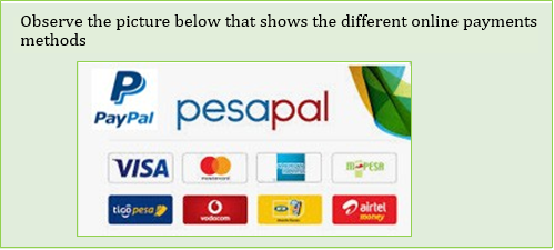
4.1.1. Online Payment methods
ACTIVITY 4.2
Answer the below questions:
1. Among the above payment method , list payment method use in Rwanda
2. Discuss steps to make payments online
Is the way that a buyer chooses to compensate the seller of a good or service that is also acceptable to the seller. Typical payment methods used in a modern business context include cash, checks, credit or debit cards, money orders, bank transfers and online payment services such as PayPal.
1. Cash Payment
Buying online requires using electronic means which are acceptable by the selling companies for example as seen in previous sections buying with Kikuu requires using MTN Money. Other online platforms may require special cards known as debit or credit cards.
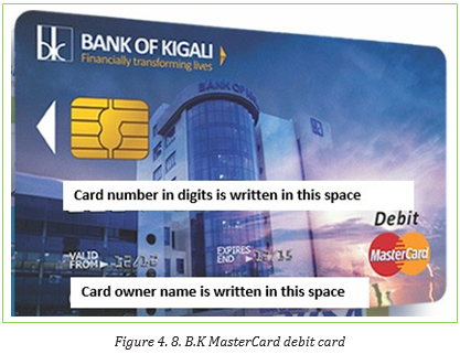
In Rwanda, banks provide means to pay using those cards. For example, Bank of Kigali provides options to buy on POS (Point of Sale) or on ecommerce platforms using Visa or MasterCard debit cards.
a. Debit & credit cards
A debit/credit card is a plastic card normally issued by a financial institution to allow its user to pay at Points of Sale in order to complete a purchase. They also allow the same purchase on online shopping platforms.
Debit and credit cards look alike and it is not easy to identify them simply by liking at them except when it is written on them. The main difference is where money is got from: for the debit cards money is immediately got from the owner bank account while for the credit card money is charged to the customer’s credit line.
The image below shows the front and back side of a credit/debit card
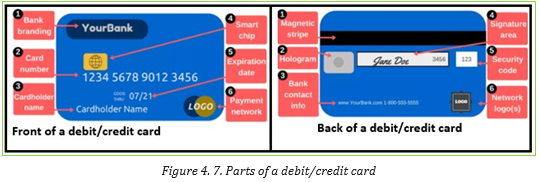
The parts found on the front side of the credit card are:
1. Bank branding which identifies the bank name that issued the card
2. Card number which is unique and identifies the client with the bank.
The card number are the ones provided while purchasing online.
Note: Keep the card number a secret as that number can be used by ill- intentioned people
3. Card holder name is the name of person authorized to use that card
4. Smart ship is the electronic circuit (processor) which stores some information. The smart ship feature makes cards more secure than the magnetic-stripe-card only
5. Expiration date is the date after which the card is no longer usable. The reason for this is mainly for the purpose of providing new cards which are more technologically advanced. The expiry date is necessary while purchasing online as most platforms require this information and when it is wrong the transaction can’t be done
6. Payment network logo is the type of card and this can be MasterCard, Visa and Discover. Services specify which types they accept for payments and knowing the card’s type is very essential.
The parts found on the back side of the credit card are:
1. Magnetic stripe: the black strip contains information about the card and its owner, and specialized devices known as card readers gather that information when the card is inserted
2. Hologram: is a mirror-like area showing a three-dimensional image that seems to move as the viewing angle changes. Holograms are security features which help merchants identify valid cards
3. Bank contact information
4. Signature panel is the place where the user’s signature is put
5. Security codes is an additional code to help ensure that anybody using the card number has a legitimate, original card
6. Network logos
An example of a typical debit card is found below
a. 1. Using a debit/credit card to purchase
The following are the steps of using a Debit/Credit card in online shopping:
1. Enter the address of the website where to purchase from in the address box of the browser’s window.
2. Select items to purchase and click the appropriate button used for purchasing the item.
3. Enter the shipping, billing and debit/credit card details.
4. Click the appropriate button to complete the transaction.
5. Print the confirmation screen or proof of purchase received upon
completing the transaction, and keep it until the item arrives.
For using debit cards at POS or ATMs insert the card and follow the prompts
b. Mobile Phone based Money
Also called Mobile money is a technology that allows people to receive, keep and spend money using a mobile phone. It’s sometimes referred to as a ‘Mobile Wallet’ or by the name of a specific service
There are more different mobile money services around the world. Although they are most popular in Africa, Asia and Latin America. Mobile money is a popular alternative to both cash and banks because it’s easy to use, secure and can be used anywhere there is a mobile phone signal.
Mobile money keeps funds in a secure electronic account linked to a mobile phone number. In some cases, the mobile money number will be the same as the phone number. Mobile money is often provided by the same companies that run the mobile phone services and it is available to both pre-pay and contract customers.
APPLICATION ACTIVITY 4.2
1. List 5 public services that are paid using Mobile money here in Rwanda
2. Discuss the payment method at your school used to pay school fees?
3. What are the advantages of Mobile money payment method over paying cash at the bank counter ?
4.2. Social media
Social media is the collective of online communications channels dedicated to community-based input, interaction, content-sharing and collaboration which enable users to create or share content or participate in social networking.
Examples of social media are: Facebook, twitter, Instagram and WhatsApp
4.2.1 FacebookACTIVITY 4.2
Facebook is one of the most popular free social networking websites. It allows registered users to create profiles, upload photos and videos, send messages and stay in touch with friends, family and colleagues.
a. Creating a facebook account
For most social media before using them an account must be created. An account
identifies the user as different from other users in the system.
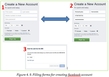
The following steps are followed to create a facebook account:
1. Open Facebook Home page by entering in the browser’s address bar the link www.facebook.com
2. The first page provides the option to login or sign up. Fill in the form the
required information and click on sign up
3. Enter personal information(First name, Last name, email or phone number, Birthday and gender)
4. Enter the code provided through SMS or the provided email
1. Open the verification email that is sent to the email provided while creating the account
2. Edit the profile information by logging into the new account and clicking on Edit profile
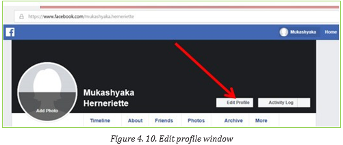
The following table will be appeared.
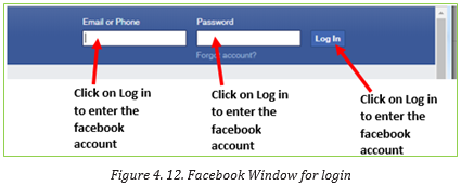
Note: The account has been created you are able to login into your facebook account:
Go to facebook.com and in the top right form fill in the email and the password then click on:
a. Connecting with friends
Facebook has millions of users, all users are in the public and appear like anonymous to you. As a facebook user you are allowed to search for other users, viewing their profiles, friends, and photos. You can immediately message them inbox but once the account owner sets some restrictions on his/her account a non-friend user may view nothing among these.
In order to be able to fully communicate with another facebook user, you just need to be a facebook friend.
To have a friend on facebook go through this process:
• In the facebook search box enter the account of the friend to be
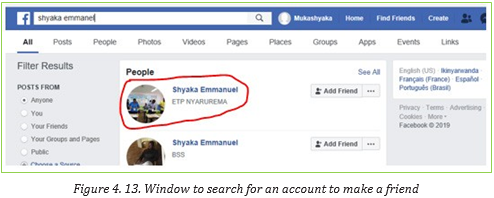
• Once the account is entered in the search box choose the correct facebook account among the many options and click Add Friend. In the image above the account chosen is Shyaka Emmanuel
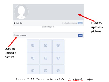
a. Sharing pictures
A facebook account holder can upload pictures on his/her facebook account, share them or share pictures uploaded by others.
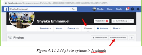
Steps to upload a picture in your account are:
• In the menu click on Photo then on Add Photos/Video
• In the new window that will appear browse for the picture to upload and open it so that it gets uploaded.
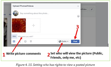
• Comment the picture, set who has rights to view it and click on Post like illustrated in the image above
The uploaded image can then be viewed by anyone (if right to view the image has been set to Public) and they can like, share and comment this image.
a. Chatting
Facebook provides the option to converse with friends by using the chat option whose window is available in the far down right zone of a facebook page.
The content of the chat is text but can be also attachments in form of text files, images, GIF files, videos or a laptop camera taken picture/video
APPLICATION ACTIVITY 4.2
1. List and explain the steps to create a facebook account
2. Create a facebook account and give it your names. Upload your picture on the account’s profile
3. Search and request for friends by focusing on your classmates
4. Chat with your friend and send them some documents related to your different subjects lessons
4.2.2. Twitter
ACTIVITY 4.4
Twitter is a free microblogging service that allows registered members to broadcast short posts called tweets. Twitter members can broadcast tweets and follow other users’ tweets by using multiple platforms and devices.
a. Creating an account
• For creating a twitter account first go enter in the browser’s address bar twitter.com
• In the first page that will appear click on Sign up. This same page is used for sign in when the user has already a twitter account
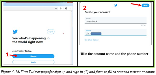
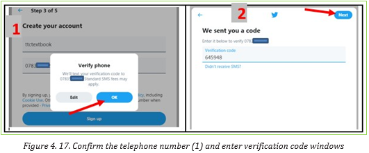
• In the next screen that will appear also click on Next. Confirm the telephone number so and use the sent code to continue to the next stage
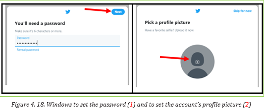
• In the next screen enter the password for your twitter account and click on Next.
The screen that will thereafter appear will allow you to edit the twitter account profile picture by clicking on the human head-and-body silhouette but this can be skipped to be done later.
In the next screens that will appear follow the prompts. Those screens will allow describing yourself, setting your interests, suggestions of accounts to follow, turning on notifications
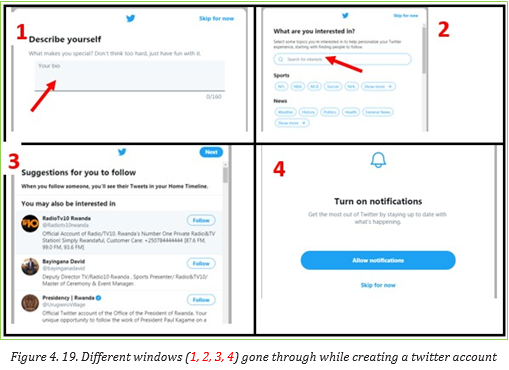
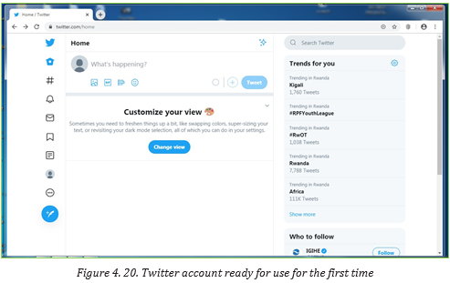
In the steps given above the account creator may decide to go into additional steps depending on which features to activate. Here most of the options have been skipped or the default provided option was chosen. After going through all the steps the account is created and is ready to be used. However the steps are subject to change and screens may not look like the ones provided here depending on changes brought in by Twitter.
a. Following a twitter account
All social media provide better experience when one is acquainted with other user in the same social media network. For a twitter user to have better experience he/she has to follow other accounts.
Following an account permits one to receive immediately prompts when the followed account posts a tweet in form of text, image or video; updates the profiles immediately after they are posted.
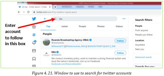
Following a twitter account is done in these steps:
1. Search for the account to follow using the twitter search box
2. Next to the searched account click on Follow. The Follow tab will immediately change into Following
C. Tweeting
Also known as tweeting is posting making a post on the social media Twitter. The post can be just text, images and videos.
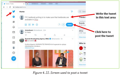
To post a tweet go through this process:
1. In the Twitter Home page click on the twitter icon
2. In the text area that will appear write the tweet text. If images and videos are to be used in the tweet click on the
corresponding icons below the text area
3. Once the tweet is ready click on Tweet. The tweet is now posted and can be viewed by the account followers and anyone
who searches for it
Note:
- witter provides the option to delete the created tweet by clicking on the drop down icon next to the tweet and clicking on Delete
- As one tweet is only of 280 character while tweeting choose properly the words to use. For this reason tweets contain more shortened words
- Twitter users can create hashtags which are keywords preceded by the hash sign and are easily searchable on twitter
D. Twitter menu icons
In the previous sections some of the available twitter options have been elaborated. Those options can however be easily accessed by using the icons located at the left side of a twitter account page. The table below represents those icons and their roles
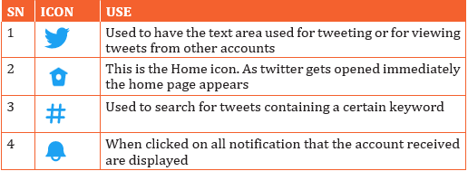
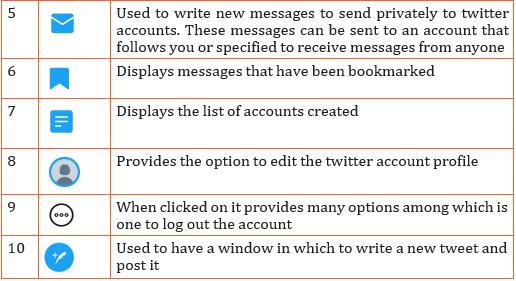
Table 4. 1. Twitter icons and their use
APPLICATION ACTIVITY 4.4
1. What is Twitter and why should you use it?
2. Create your twitter account and do the following:
a. Make it have your picture as a profile picture
b. Search for accounts to follow mainly your classmates
c. Post some tweets about your school and lessons
4.2.3. Instagram
ACTIVITY 4.5
Instagram is one of the Social media platform used by many people:
a. Discuss the use of Instagram
b. Do a research and differentiate Instagram from other social media namely facebook and Twitter
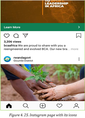
Analyze the Instagram icon and discuss how it relates Instagram useInstagram is a free social networking service built around sharing photos and videos. It launched in October 2010 on iOS (iPhone Operating Systems) first, and became available on Android in April 2012 and can be accessed via computer internet browsers.
Similar to Facebook or Twitter, everyone who creates an Instagram account has a profile and a news feed. When a photo or video is posted on Instagram it will be displayed on the account’s profile and accounts that follow you will see it in their own feed. Likewise posts from other accounts can be viewed if you chose to follow them.
Just like other social networks, an account can interact with others on Instagram by following them, being followed by them, commenting, liking, tagging.
a. Creating an Account on Instagram
Like other social media one cannot use Instagram without having an account created and for that go through these steps:
1. Enter in the browser’s address bar the URL of the application (instagram. com)
2. In the form that appear to the right of the new page fill in the required
details and click on Sign up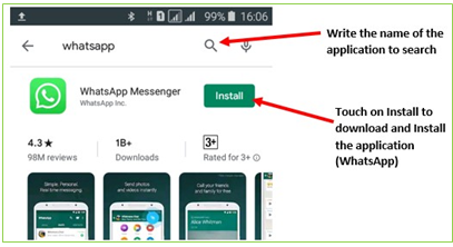
3. in the next screen click on Turn on (to turn on notification) or Not so as to be directed to the Instagram first page
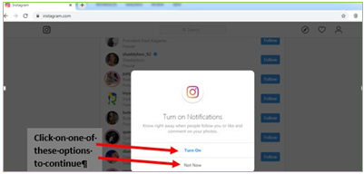
Figure 4. 24. Window to turn on notifications and have access to other accounts
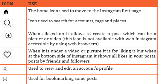
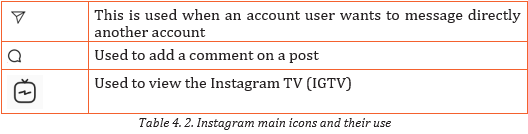
d. Instagram main icons
Instagram has got icons which help carry out the basic functions. Those icons are shown in the image below:
The role of each icon is explained in the table below:
APPLICATION ACTIVITY 4.5
1. Create an Instagram account under your name
2. Follow some of your class mates
3. Create posts and comment posts from other accounts
4.2.4. WhatsApp
Umurerwa, a grade 2 student, has heard of a phone application that she can use to chat, send a photo and video call. She decided to use her father’s phone to find this app.
Observe the screen of Umurerwa‘s father
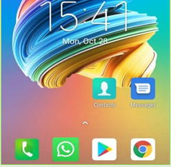
Answer the below questions:
1. Among these applications, which application Umurerwa should use?
2. Explain why you have chosen that application
WhatsApp is a popular messaging app with end-to-end encrypted instant messaging that can be used on various platforms, including Android, iPhone and Windows smartphones, and Mac or Windows PCs.
For WhatsApp to be installed on PCs an auxiliary application is needed in order to create a virtual environment resembling a Mobile Operating System in which WhatsApp will be installed. Such auxiliary applications are NoxPlayer and Blue Stack.
A. Installing WhatsApp
Installing WhatsApp first requires downloading it through the phone application for downloading applications. For android that application is Play Store. Download WhatsApp by searching for it in Play Store and install it by going through the prompts

Figure 4. 26. Android phone window for downloading and installing applications (WhatsApp)
In the next screen that will appear touch on Accept and let the application download. When there is not enough space for downloading the application, it will be necessary to delete some files to liberate some space.
Downloading and installing WhatsApp will go through these steps shown in the screenshots below:
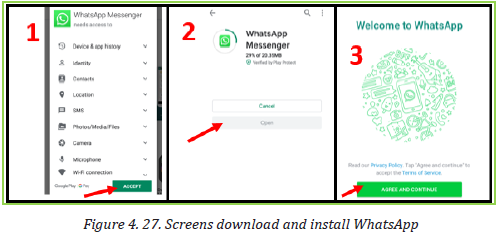
Interpretation of the screens:
a. Screen One: The choosing of the application to download and install has already been done now the person has to agree that WhatsApp will have rights to have access to some of the resources in the telephone.
b. Screen Two: WhatsApp is now being downloaded and is at 26%. Once downloading is over the application will install itself and when finished the user will touch on Open to do further configurations.
c. Screen Three: Once the Open option is touched in the next screen touch on Agree and Continue to agree to the terms of service.
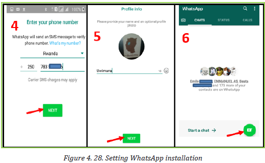
d. Screen Four: In this screen fill in the phone number to use on WhatsApp and touch on Next. A WhatsApp code message will be sent to your telephone. Enter it in the next screen and continue
e. Screen Five: Configure WhatsApp by uploading an image that will be used as a profile picture to your account and set the account name.
f. Screen Six: WhatsApp is now installed. Start chatting by touching on the icon shown by an arrow.
B. Adding a Status in WhatsApp for Android
Similar to apps like Snapchat and Instagram, WhatsApp Status is a place for snapping pictures of whatever you’re doing and then uploading them to your profile where they’re available for your contacts to see for 24 hours.
To getstarted with Status:
- Tap the Status bar on the home screen.
- Tap the camera icon at the bottom-right.
- Take a picture or video.
- Add any filters, stickers, text, or whatever else you’d like.
- Tap the green circle at the bottom-right to add the post to your Status.
APPLICATION ACTIVITY 4.6
1. Discuss the improvement WhatsApp has brought in the communication area in Rwanda
2. Compare options provided by WhatsApp and Instagram
4.3. Online Services
An online service refers to any information and services provided over the Internet.
These services not only allow subscribers to communicate with each other, but they also provide unlimited access to information. Online services may include E Banking, E payment, etc
4.3.1. E-Banking and E-Payment
ACTIVITY 4.7
Read the scenario below:
During the weekend, Kamana was sent home for school fees issues but on Monday, 7:30 AM he must attend the exam after the payment of the school fees. Umwalimu Sacco Cooperative where Kamana’s parents keep their money did not open as it was on Sunday.
Answer the questions below:
1. What Kamana should do to not miss the exam?
2. Give examples of services that can be paid electronically in Rwanda
E-Banking and E-Payment
It is an electronic transfer of money from bank account, usually checking account without the use of the paper check. E-cash is a form of an Electronic payment system where a certain amount of money is stored on client’s device and made accessible for online transaction.
a. E Banking
Electronic banking is a form of banking in which funds are transferred through an exchange of electronic signals rather than through an exchange of cash, checks, or other types of paper documents
It is also a method of banking in which the customer conducts transactions electronically via the Internet.
Transfer of funds occur between financial institutions such as banks and credit unions. They also occur between financial institutions and commercial institutions such as stores. Whenever someone withdraws cash from an Automated Teller Machine (ATM) or pays for services using a debit card, the funds are transferred via electronic banking.
E-banking is a safe, fast, easy and efficient electronic service that enables an access to a bank account and to carry out online banking services, 24 hours a day, and 7 days a week.
With this service you save your time by carrying out banking transactions at any place and at any time, from home or office provided there is internet access.
E-banking enables the following:
- Accurate statement of all means available in your bank account
- Statement of current account, credits, overdrafts and your deposits
- Execution of national and international transfers in various currencies
- Execution of all types of utility bill payments (electricity, water supply, telephone bills, and many others)
- Carrying out customs payments
- Electronic confirmation for all transactions executed by E-banking
- Management of your credit cards
Disadvantages
The disadvantages presented by E-banking are linked to the fact that it is a new technology which is not usable by anyone especially in countries where ICT literacy is still a problem.
Other disadvantages are also linked to weaknesses in the system that may be exploited by hackers who may steel money using weaknesses found in the system
b. E payment
An e-payment system is a way of making transactions or paying for goods and services through an electronic medium, without the use of checks or cash. It’s also called an electronic payment system or online payment system. E-payment includes the use of Debit/credit card, Mobile Money
Services done by mobile money
Services provided by Mobile Money include money transactions whereby money can be sent from one telephone user to another who can then withdraw the money as cash or keep it and use to pay for different goods and services.
Example
In Rwanda mobile money services are provided by TIGO Cash, MTN Mobile Money and Airtel Money. They include money transfer and withdrawal from a mobile money account and from even a bank account, payment of different bills like water and electricity.
APPLICATION ACTIVITY 4.7
1. Give 3 differences between credit card payment and mobile money payment
2. By conducting a research on the Internet, analyze the Rwandan context in terms of electronic payment. Give the benefits to
Rwandans if the country adopts electronic payment in all transactions.
4.3.2. Irembo local online services
ACTIVITY 4.8
By searching the Internet, list the services available for Irembo.rw and analyze them if they meet the expectations of the local population.
Irembo is an initiative by the Government of Rwanda aiming at improving its service delivery to the citizens and businesses. Irembo is the one-stop portal for e-Government services. Irembo as a platform has the role of the provision of Government services online with ease, efficiency and reliability.
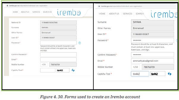
How to create account from irembo
- Type www.irembo.gov.rw in the address bar of your browser
Fill in dialogue box black space
a. Password place
b. Confirm Password
c. Email
d. Captcha Text
These services are subject to changes as some services can be added but the ultimate goals is to have all services offered through this platform.
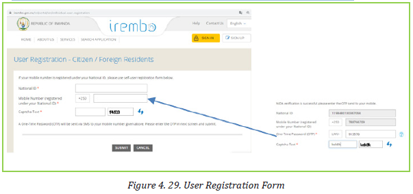
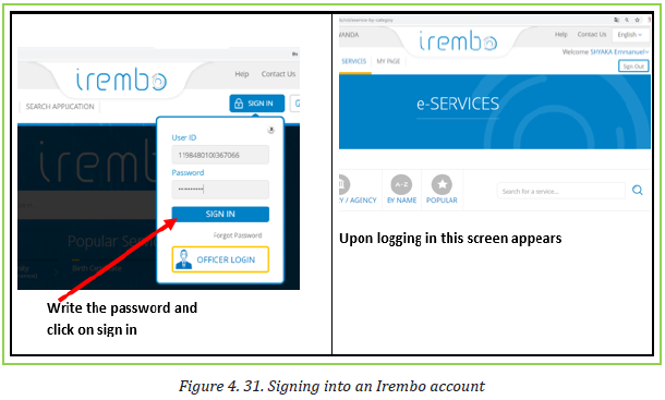
a. Requesting for Irembo service
Requesting for services on Irembo requires first to have a username which is the identity card number without the last three digits and a password
b. Current Irembo services
Currently, Irembo services are into these categories:
1. Immigration and emigration
2. Land
3. Local government
4. National ID
5. Notarization and Gazette services
6. Police
7. Rwandans living abroad
8. Media
9. Education
10. Health
11. Ubudehe and mutuelle
12. Institutions of national meseum of Rwanda
13. Transportation
14. Tourism
Requesting for a criminal records clearance
1. Open irembo website
2. Enter your ID and Password
3. Payment using VISA, MasterCard , MTN Mobile money(*182#), airtel (*182#), Tigo(*310#) Mobicash or BK
4. After paying you send sms/email confirming that you have requested a service and service paid
5. Feedback of certificate must be sent to you after 3 days
Advantages of using irembo
1. Helps citizens to save a time
2. Save transport
3. People can request a service when he or she is at home
4. Reducing corruption malpractices
5. It creates jobs
6. It simplifies access to the Government services
7. Avoiding friendship
APPLICATION ACTIVITY 4.8
1. List and explain 5 advantages of using IREMBO Service
2. Explain at least 3 problems that Irembo services have come to solve
END UNIT ASSESSMENT
1. Give the difference between WhatsApp , Instagram and Twitter ?
2. Using a clear example, explain 3 common features of social media
3. Give examples of services that can be paid electronically in Rwanda
4. Give 3 differences between credit card payment and mobile money.
BIBLIOGRAPHY
1. National Curriculum Development Centre (NCDC). (2011). ICT Syllabus for Upper Secondary. Kigali.
2. MYICT. (2011). National ICT strategy and plan NICI III-2015.Kigali.
3. National Curriculum Development Centre (NCDC). (2006). ICT syllabus for Lower Secondary Education. Kigali.
4. Pearson Education. (2010). Computer Concepts.
5. Rwanda Education Board (REB), (2019), ICT Syllabus for TTC, (2019), Kigali
6. Rwanda Education Board (REB) (2019), Computer Science S5 student’s book
7. Rwanda Education Board (REB) (2019), Computer Science S6 student’s book
8. Rwanda Education Board (REB) (2019), Information and Communication Technology for Rwandan Schools Secondary 1 Students’ Book
9. Rwanda Education Board (REB) (2019), Information and Communication
Technology for Rwandan Schools Secondary 1 Students’ Book
10. Rwanda Education Board (REB) (2019), Information and Communication
Technology for Rwandan Schools Secondary 2 Students’ Book
11. Longhorn Publishers (2016) Computer Science For Rwandan Schools Senior Four Student’s Book
12. Fountain Publishers (2016) Information and Communication Technology (ICT) for Rwanda Schools Learner’s Book Senior Three
13. https://www.bigcommerce.com