UNIT 1: ADVANCED SPREAEDSHEET II
Key Unit competence: Use the full potential of the spreadsheet to manipulate data.
1.0 INTRODUCTORY ACTIVITY
1. Using Ms Excel summarize the number of expectant mothers and children under 2 years in the cells of Muhororo Sector who must receive mosquito nets
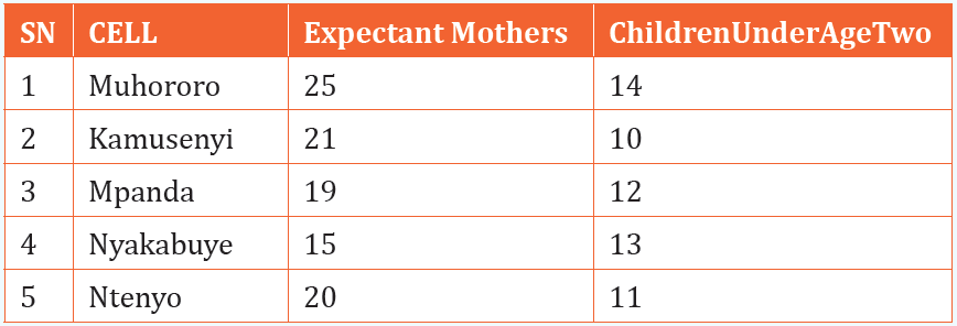
a. Which cell that has more expectant mothers to receive mosquito nets?
b. Which cell that has more children under age Two?
c. Calculate the average number of children to receive mosquito nets in Muhororo
d. Which cell has less children under age Two?
1.1. Advanced Spreadsheet functions
1.1.1. Logical functions
ACTIVITY 1.1
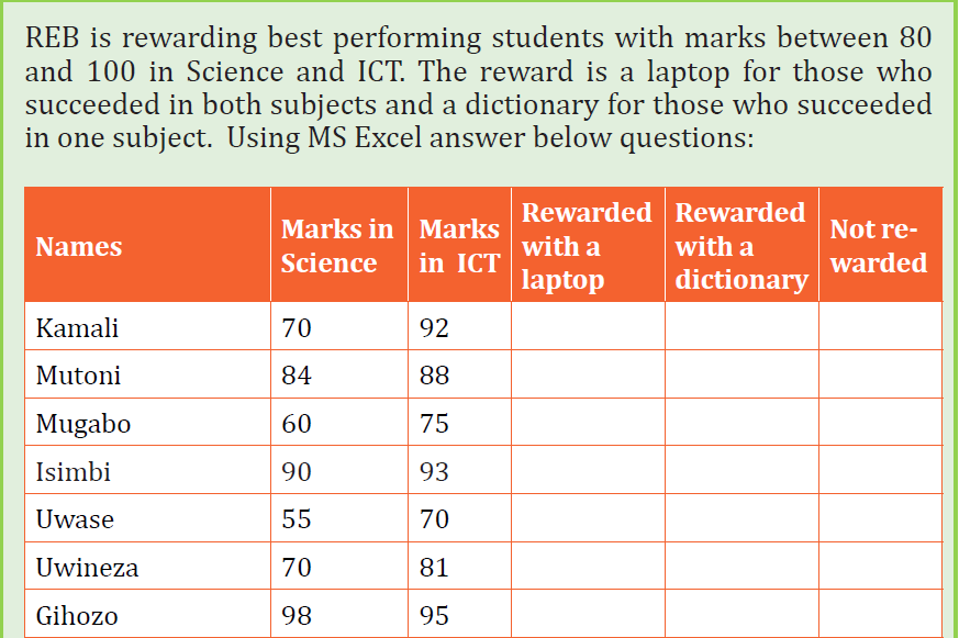

a. Write an Excel function to find students who are to be rewarded with laptops, dictionaries and those not rewarded
b. Determine the number of students that have not been rewarded?
c. How many laptops and dictionaries will be given?
d. In which subject does Kamali have more marks?
e. In which subject does Mutoni have minimum marks
f. Use Excel logical functions to fill the table above
A condition is an expression that either evaluates to true or false. The expression could be a function that determines if the value entered in a cell is of numeric or text data type, if a value is greater than, equal to or less than a specified value, etc.
Logical Function is a feature in Excel that allows excel users to introduce automated decision-making when executing formulas and functions.
The role of functions in this is to check if a condition is true or false. It combines multiple conditions together and comes up with a result depending on the result of the evaluation of the condition.
a. IF Function
The If function checks whether data in a cell meets a certain condition and returns one value which can be True or False
- Syntax: = IF(Logical_test, Value_If_True, Value_If_False )
The If function takes as arguments the logical test, checks if it evaluates to true and if so returns as a result the content of the second argument and if false the content of third argument is returned
- Example 1:
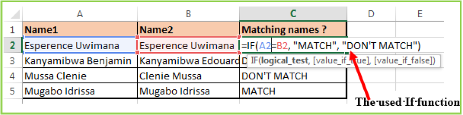
Figure 1. 1. The use of If function to compare names
In the above example the If function with its arguments is entered in the cell where the result is to appear.
To apply that function in other cells proceed like this:
1. Place the cursor in the bottom corner of the cell
2. Hold down the left key, scroll down to other cells and release the left button
The If function in the above examples checks if the two names are alike and if yes, the function writes MATCH in the cell, if not the function writes DON’T MATCH
• Example 2:
Considering the marks obtained by Irasubiza, Karenzi, Byukusenge and Shyaka in ICT, Maths and English. The If function checks if the marks are greater than 87 and gives to the candidate the Very Good note else the Good note is given.
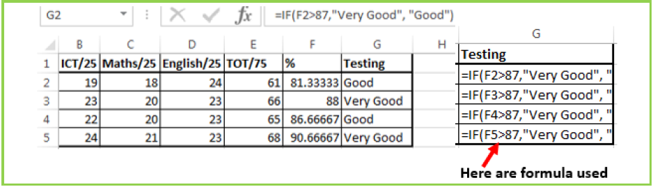
Figure 1. 2. Use of if function to award grades
b. AND Function
The Excel AND function is a logical function used to test if two or many conditions are true. The result is TRUE if all the conditions are true else the result is FALSE
- Syntax: =AND (Logical1, Logical2, logical3,…)
- Example:
In the table below the And function checks if people in the table studied
Education and that their age is greater than 18
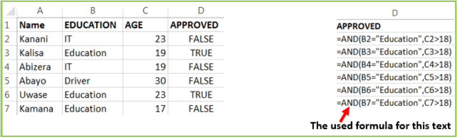
Figure 1. 3. Results of And function and on the left functions used
Note: the And function may have more than two arguments and for the results to be True all the arguments must evaluate to TRUE and if one of the arguments is false all the result is FALSE
Interpretation of the results:
The second, fourth, fifth and seventh rows evaluate to True as the education for all those rows is Education and the age is greater than 18 while the remaining rows evaluate to FALSE as they don’t meet the two criteria.
c. FALSE Function
The FALSE function takes no arguments and generates the Boolean value FALSE.
It is used to compare the results of a condition or function that either returns true or false
- Syntax: =False
The false function takes no argument but just returns the logical value False
- Example: The False function used in the example below returns FALSE if the age entered in C2 is less than 10 (C2<10)
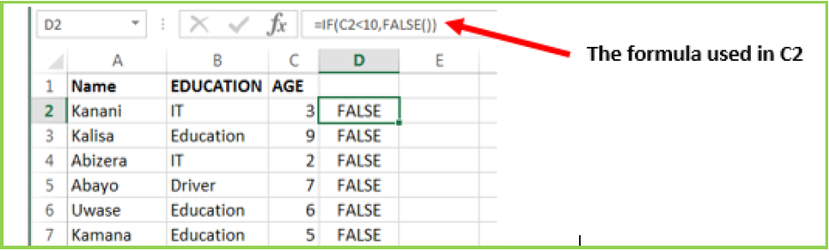
Figure 1. 4. The use of the False function in Excel
Interpretation:
The used function “=IF(C2<10,FALSE
)” will check if the C2 cell data is less than 10, if so it will return False as a result else it will return True. The same function will be applied to other cells by changing the cell position
d. NOT Function
The Excel NOT function returns the opposite of a given logical or Boolean value. When given TRUE, NOT returns FALSE. When given FALSE, NOT returns TRUE. Use the NOT function to reverse a logical value.
- Syntax: =NOT(Logical)
The not function takes one logical expression as an argument. It returns an error if more than one argument is used.
- Example
The table below will have all its content returned to True by the use of the NOT function. If the results to reverse were got by using a formula the Not function can be put in front of the function/formula to make the latter an argument of the Not function.
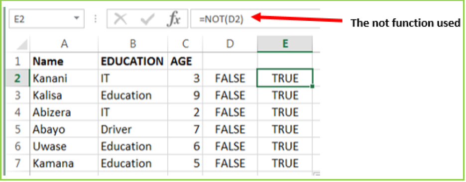
Figure 1. 5. Not function and its results
Note: If the results in column D2 were got by using the function
“=IF(C2<10,FALSE
“=NOT(IF(C2<10,FALSE
e. The OR function
The OR function is a logical function to test multiple conditions at the same time. OR returns either TRUE or FALSE.
- Syntax: = OR(logical1, Logical2, …)
- Example:
The OR function in the screenshot below checks for students who got more than 70% as the Pass mark in anyone of the three tests.
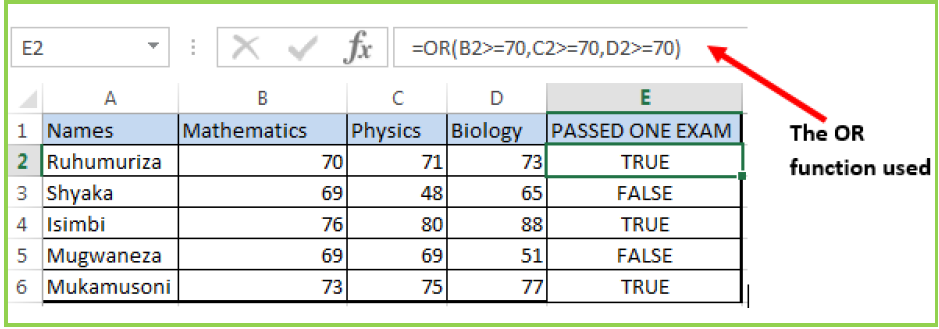
Figure 1. 6. The OR function to test if any of the arguments is true
APPLICATION ACTIVITY 1.1
1. Give the difference between IF and AND functions?
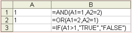
2. Which of these three functions in column B will give you TRUE as an answer?
1.1.2. Advanced Math Spreadsheet functions
ACTIVITY 1.2
You are given the following data in Microsoft Excel data sheet.
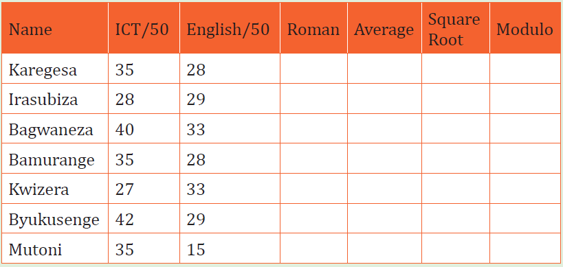
Answer below questions:
1. Convert ICT marks into Roman style?
2. Discuss on how to calculate the modulus of the students’ marks?
3. Calculate the square root of student average marks?
4. Discuss the conversion from roman style to Arabic style number?
Mathematical functions are used to calculate values basing on what is in cells, perform operations on a cell content, fetch values after an operation based on the search criteria and much more. Some of the functions to be seen here are
Abs
a. ABS
The Excel ABS function returns the absolute value of any provided number.
The syntax of the function is: ABS (number)
Where the numerical argument is the positive or negative numeric value for which the absolute value is to be calculated.
Examples:
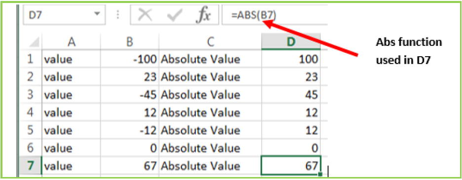
Figure 1. 7. Example of the use of Abs Function
b. ARABIC
The Excel Arabic function converts a Roman numeral into an Arabic numeral.
The syntax of the function is: ARABIC (text)
Where the text argument is a text representation of a Roman numeral not exceeding 255 characters.
Note that:
- If supplied directly to the function, the text argument must be encased in quotation marks;
- If an empty text string is supplied, the Arabic function returns the value 0;
- The Arabic function was only introduced in Excel 2013 and so is not available in earlier versions of Excel.
Below are five examples of converting ARABIC to NUMBERS
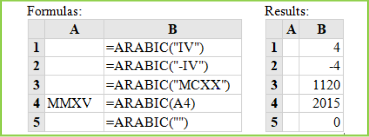
Figure 1. 8. Results of using an Arabic function
c. ROMAN
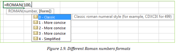
The Excel ROMAN function converts an Arabic number to a Roman number.
This means that if a function is supplied with an integer, the function returns a text string showing the Roman numeral form of the number.
The syntax of the function is: ROMAN (Number, [form])
- Where Number is any Arabic number and the form specifies the presentation format of the Roman number to be calculated. The formats to choose from are displayed after writing the number to convert and writing the comma but the default (classic) is used.
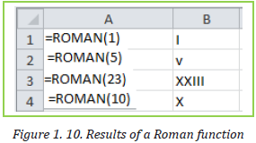
- Roman Function use examples
In the following spreadsheet, the Excel Roman function is used to convert the number 1999 to different forms of Roman numerals.
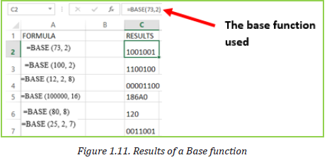
d. BASE
The Excel Base function converts a number into a supplied base and returns a text representation of the calculated value. The Base function was introduced in Ms Excel 2013 and therefore, it is not available in earlier versions of Excel.
The spreadsheet below shows three examples of the Excel Base Function.
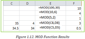
e. MOD
The Excel MOD function returns the remainder of a division between two supplied numbers.
The syntax of the function is: =MOD (number, divisor)
The spreadsheet below shows four simple examples of the Excel Mod function.
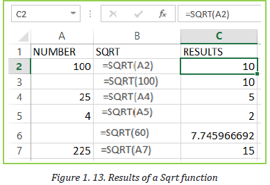
f. SQRT
The Excel SQRT Function calculates the positive square root of a supplied number.
The syntax of the function is: SQRT (number)
- Where the number argument is the numeric value for which the square root is to be found.
If the supplied number is negative, the Sqrt function returns the #NUM! Error.
- Excel Sqrt Function Examples
The following spreadsheet shows three simple examples of the Excel Sqrt function
.APPLICATION ACTIVITY 1.2
1. What is the difference between MOD and SQRT Functions
2. Using Excel change the following Roman into Arabic style
a. MCCIII
b. XLIX
c. CMV
d. XXIII
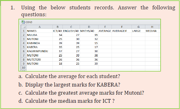
1.1.3. Advanced Statistical Spreadsheet functions
ACTIVITY 1.3
The table below contains students’ marks.
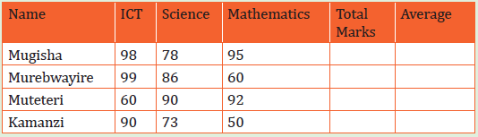
Answer the questions that follow:
a. Calculate the average marks of every student
b. Give the name of the one who has more marks in:
i. ICT
ii. Science
iii. Mathematics
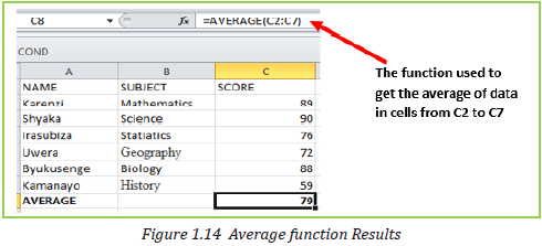
a. AVERAGE
The AVERAGE function in Excel returns the arithmetic mean of a list of supplied numbers, where the number arguments are a set of one or more numeric values, or arrays of numeric values, for which the average is to be calculated.
- Syntax of AVERAGE Function in Excel = Average (Number1, Number2,…)
An example of how Average function is used is displayed in the screenshot below:
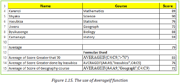
b. AVERAGEIF
AVERAGEIF Function in Excel finds and returns the average of array that meets the specific condition. The AVERAGEIF function in Excel supports logical operators (>, <, <>, =)
- Syntax of AVERAGEIF Function in Excel: =AVERAGEIF (range, criteria, [average_range])
Where:
- Range: An Array of range to be tested against the supplied criteria.
- Criteria: The criteria or condition on which average has to be calculated.
- [average_range]: An optional array of numeric values for which the average is to be calculated.
Example of AVERAGEIF Function in Excel
In the Excel screenshot below the averages of cells meeting certain conditions have been calculated. Those conditions are: cells with scores greater than 70, average for Irasubiza and average for science courses.
c. LARGE
The LARGE Function in Excel returns the largest value from an array of numeric values.
- The syntax of LARGE Function is =LARGE (array, k)
Where:
- Array – An array of numeric values from which to find the Kth largest value.
- K- The index. Value of K that is passed to find the Kth largest value.
Example of LARGE Function in Excel:
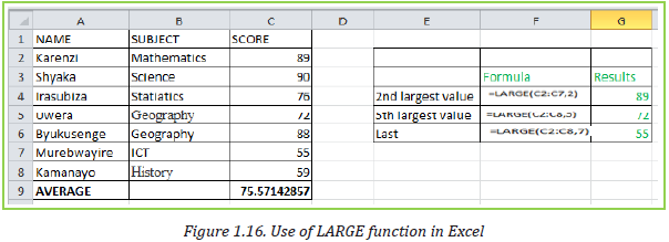
Interpretation:
- First Example finds the 2nd Largest Value as 89
- Second Example finds the 5th Largest Value as 72
- Third Example finds the 7th Largest Value as 55
d. MAXIFS
MAXIFS function in Excel returns the Maximum value from the set of supplied numbers that meets some specific conditions. In other terms it returns the maximum if a condition is met. The MAXIFS function in Excel supports logical operators (>, <, <>, =) and wildcards characters (*,) for pattern matching. Syntax of MAXIFS Function in Excel:
- MAXIFS( max_range, criteria_range1, criteria1, [criteria_range2, criteria2], … )
Where:
- max_range: is the range of numeric values from which to find the maximum value if the conditions are satisfied.
- criteria_range1: is an array of values to be tested against the criteria “criteria1”.
- criteria1: is the condition to be tested against the values in criteria_ range1
Example of MAXIFS Function in Excel
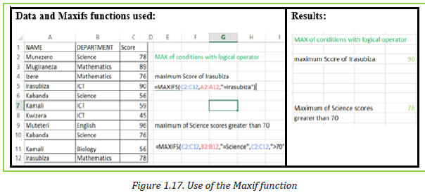
- First two examples states the use of logical operation in MAXIFS function with conditions.
- Last two examples states the use of wildcards in MAXIFS function with two conditions.
e. MEDIAN
MEDIAN function in Excel returns the statistical median or middle value of a list of supplied numbers.
Syntax of MEDIAN Function in Excel is: = MEDIAN (number1, [number2], …)
Where the number arguments are a set of one or more numeric values for which to calculate the median.
An example of how the Median function is used in Excel is shown in the table below:
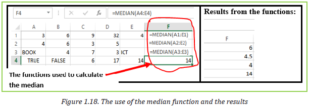
- When the total number of supplied values is odd, the median is calculated as the middle number in the group.
- When the total number of supplied values is even, the median is calculated as the average of the two numbers in the middle.
- Cells containing Text values, logical values, or no value are ignored.
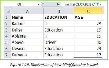
f. MINIF Function
The Excel MINIFS function returns the smallest numeric value that meets one or more criteria in a range of values. MINIFS can be used with criteria based on dates, numbers, text and other conditions.
Syntax:
g. MODE Function
MODE function in Excel returns the mode which is the most frequently occurring number in a group of supplied arguments.
The Syntax of MODE Function in Excel is =MODE (number1, [number2],…)
Where the number of arguments are a set of one or more numeric values for which you want to calculate the mode.
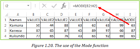
Cells containing Text values, logical values, or no value are ignored.
- Mode (most frequently occurring value) is calculated row wise in above example.
APPLICATION ACTIVITY 1.3
1.1.4. Text spreadsheet functions
ACTIVITY 1.4
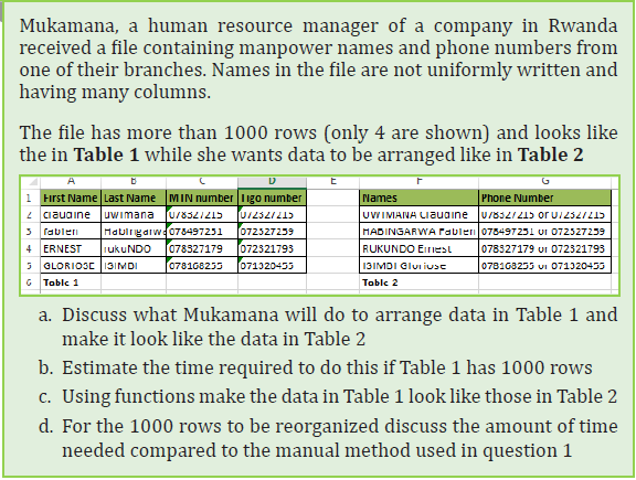
Excel has functions which facilitate an automatic manipulation of text which would take too much time if it was done manually.
For example in the case presented in the activity above if one has to combine data from two rows into one for a total of 1000 rows by copying data from one row and pasting it next to data in the other row and if one can do one row in 2 seconds, the whole exercise would take up to 33 minutes. Considering that some names which are in upper case must be in lower case and some in lower must be in upper which would require rewriting the names the whole exercise can take up to an hour.
That is where Excel ingeniosity comes in by providing functions which can allow one to do this in less than one minute. The section below explore the functions that can be used to do such a task
a. CHAR
The CHAR function returns the character based on the ASCII value. The CHAR function is a built-in function in Excel that is categorized as a String/Text Function.
The syntax for the CHAR function is:
- CHAR( ascii_value )
The ASCII value is used to retrieve the character.
Example: Explore how to use the CHAR function as a worksheet function in Microsoft Excel:
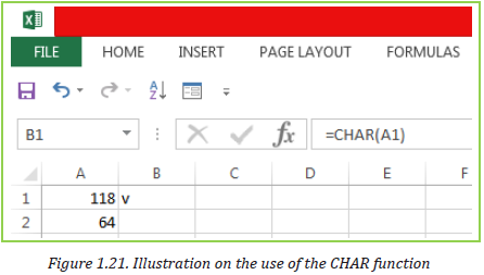
Based on the Excel spreadsheet above, the following use of the CHAR function would return:
=CHAR(A1) : Gives Result: “v”
=CHAR(A2) : Gives Result: “@”
=CHAR(72) : Gives Result: “H”
=CHAR(109) : Gives Result: “m”
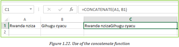
b. CONCATENATE
The CONCATENATE function in Excel is designed to join different pieces of text
together or combine values from several cells into one cell.
The syntax of Excel CONCATENATE is as follows:
CONCATENATE (text1, [text2], …)
Where text is a text string, cell reference or formula-driven value.
Below is an example of using the CONCATENATE function in Excel in which data from two cells has been combined.
The simplest CONCATENATE formula to combine the values of cells A1 and B1 is as follows:
=CONCATENATE(A1, B1)
c. UPPER
The UPPER function is a built-in function in Excel that is categorized as a String/
Text Function. It converts a text (String) into uppercase
Example:
A1==” better technology for the best future” =UPPER(A1)
Result: “BETTER TECHNOLOGY FOR THE BEST FUTURE”
d. LOWER
The LOWER function is used to convert text (String) into small cap text
Example: B1=”EXCEL SCIENCES THROUGH TECHNOLOGY” =LOWER (B1)
Result: excel sciences through technology
APPLICATION ACTIVITY 1.4
1.2. Using formula & functions from different sheets
ACTIVITY 1.5
When the workbook has many sheets there is a possibility to get data from one sheet into another by using formula or functions.
Example 1:
Consider the example below which are data from two different sheets named Sheet1 and Sheet2. These sheets contain marks for ICT and for Biology. The teacher wants to make totals for each student for the two subjects and keep those totals in a separate sheet “Sheet3”
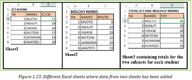
To achieve this go to the table in Sheet3 where totals of data from the two sheets
has to be done then in the TOT column cell C3 write the formula to use which is =Sheet1!C3+Sheet2!C3
Meaning that data from cell C3 of Sheet1 is added to data from cell C3 of sheet2
You can do this by writing formula from scratch or by:
- Writing the equal sign in the cell where total is to be written
- Going to the cell containing the first data to be added and selecting it
- Writing the + sign
- Selecting second data to be added by going to the sheet containing that data and selecting the right cell and lastly hitting enter
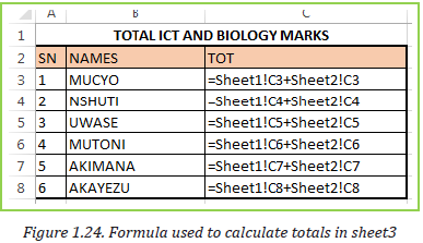
The formulas used to calculate the totals for the example above are in the image below:
Example 2:
Consider another example in which two sheets Sheet1 and Sheet2 contains data (score) on different subjects. The average of marks contained in the two sheets is going to be calculated and kept in Sheet1. The formula used is
=AVERAGE(C2:C10,Sheet2!C2:C10)
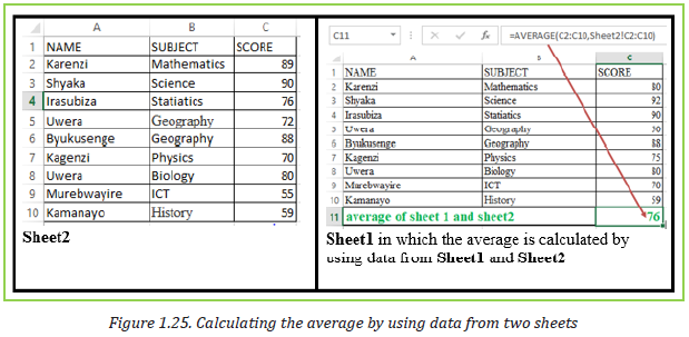
Consider the screenshots of excel tables containing data from the three sheets Sheet1, Sheet2 and Sheet3
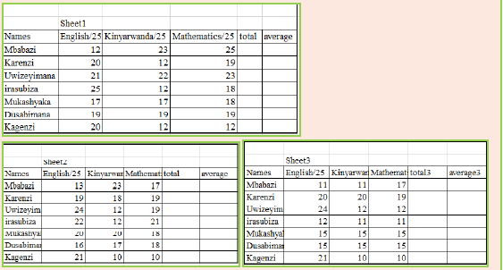
a. Calculate the total and average of every student per sheet
b. Calculate the total1, total 2 and total 3 into total 3 of the third sheet
c. Calculate the average1, average 2 and average 3 into average 3 of the third sheet
1.3. Protecting worksheet style, contents and elements
ACTIVITY 1.6
At the end of the school year, GS Kamucyo teachers receive student reports so that they may fill in marks for the third term , do totals and average for the whole year. However the head teacher fears that teachers may mistakenly change even marks for Term I and Term II
a. Which advice would you give to the head teacher on what to do in order to avoid this?
b. If this advice is adopted, teachers won’t be able to edit term I and
II. What can be done to allow them to do it if it is found necessary?
1.3.1. Protecting & unprotecting worksheet;
Worksheet protection is to prevent other users from accidentally or deliberately changing, moving, or deleting data in a worksheet, you can lock the cells on your Excel worksheet and then protect the sheet with a password.
With worksheet protection, you can make only certain parts of the sheet editable and users will not be able to modify data in any other region in the sheet.
Rules to follow for protecting worksheets with strong protection
a. Protect your sheets with strong passwords that include different types of alpha numeric characters and special symbols. At that, try to make passwords as random as possible
b. Protect the workbook structure to prevent other people from adding, moving, renaming or deleting the sheets.
c. For workbook-level security, encrypt the workbook with different passwords from opening and modifying.
d. If possible, store your Excel files with sensitive information in a secure location, e.g. on an encrypted hard drive.
To protect a sheet in Excel 2016, 2013 and 2010, perform the following steps.
a. Under the Review tab click on Protect Sheet.
b. Type the password and click on Ok
c. Reenter password and click on Ok
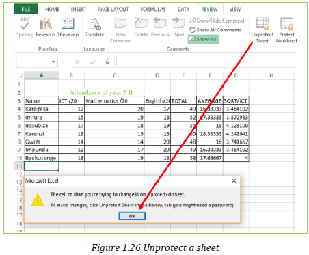
When a sheet is protected, anyone will be able to read data but will not be able to modify it and once data in that sheet is modified this message below will be displayed
1.3.2. Lock &unlock cells, style, contents and other elements
a. How to Lock Cells for Editing and Protect Formulas
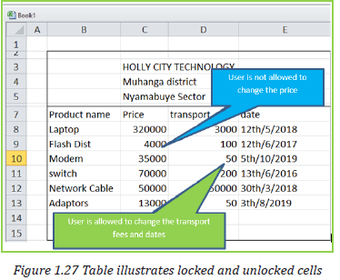
When a sheet is shared while some sheet cells must not be modified some rules have to be set so that data can be modified by anyone who wants it but not modified by someone who does not have the right to do so. In the table below a list of products will be sent to the customers. Customers will be able to modify some product records.
The great news is that you can lock cell, or a whole range of cells, to keep your
work protected. Here’s how to prevent users from changing some cells.
Type a password in the corresponding field.
Be sure to remember the password or store it in a safe location because you will need it later to unprotect the sheet.
Select locked cells .
If only these two options are selected, the users of your sheet, including yourself, will be able only to select cells (both locked and unlocked).
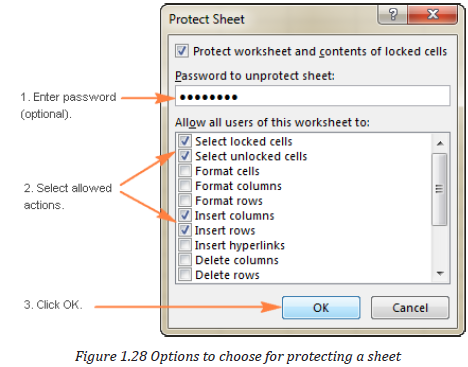
If the worksheet protection is nothing more than a precaution against accidental modification of the sheet contents by yourself or by the members of your local team, you may not want to bother about memorizing the password and leave the password field empty
Select the actions you allow the users to perform.
b. How to unprotect Excel sheet with password
To lock only specific cells and ranges in a protected worksheet
Follow these steps:
1. Select the cells you want to lock.
2. On the Home tab, in the Alignment group, click the small arrow to open the Format Cells popup window.
3. On the Protection tab, select the Locked check box, and then click OK to close the popup.
4. Right-click the sheet tab, and select Unprotect Sheet from the context menu.
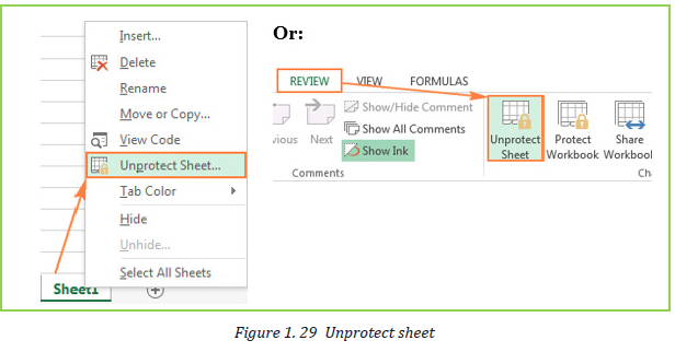
On the Review tab, in the Changes group, click Unprotect Sheet.
- On the Home tab, in the Cells group, click Format, and select Unprotect Sheet from the drop-down menu.
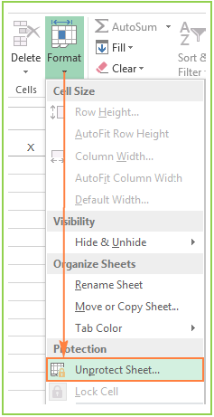
Figure 1.30. Unprotect sheet second method
APPLICATION ACTIVITY 1.6
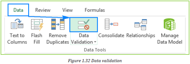
1.4. Data validation
ACTIVITY 1.7
Excel Data Validation is a feature that restricts (validates) user input to a worksheet. Technically, you create a validation rule that controls what kind of data can be entered into a certain cell.
Here are just a few examples of what Excel’s data validation can do:
- Allow only numeric or text values in a cell.
- Allow only numbers within a specified range.
- Allow data entries of a specific length.
- Restrict dates and times outside a given time frame.
- Restrict entries to a selection from a drop-down list.
- Validate an entry based on another cell.
- Show an input message when the user selects a cell.
- Show a warning message when incorrect data has been entered.
- Find incorrect entries in validated cells.
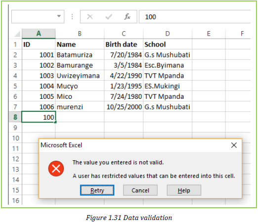
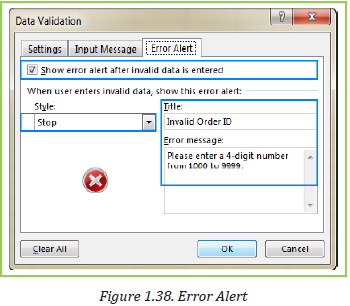
For instance, you can set up a rule that limits data entry to 4-digit numbers between 1000 and 9999. If the user types something different, Excel will show an error alert explaining what they have done wrong. The window below shows a warning message that appears when data outside of the range (1000-9999) is entered.
How to do data validation in Excel
1. Select the cell(s) you want to create a rule for.
2. Select Data >Data Validation.
3. On the Settings tab, under Allow, select an option.
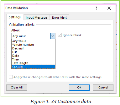
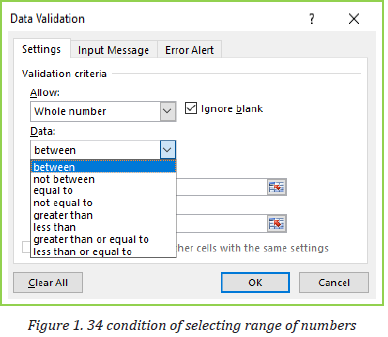
4. Under Data, select a condition:
5. On the Settings tab, under Allow, select an option:
6. Set the other required values, based on what you chose for Allow and Data. For example, if you select between,
then select the Minimum: and maximum: values for the cell(s).
7. Select the Ignore blank checkbox if you want to ignore blank spaces.
8. If you want to add a Title and message for your rule, select the Input Message tab, and then type a title and input message.
9. Select the Show input message when cell is selected checkbox to display the message when the user selects or hovers over the selected cell(s).
10. Select OK.
As an example, let’s make a rule that restricts users to entering a whole number between 1000 and 9999:
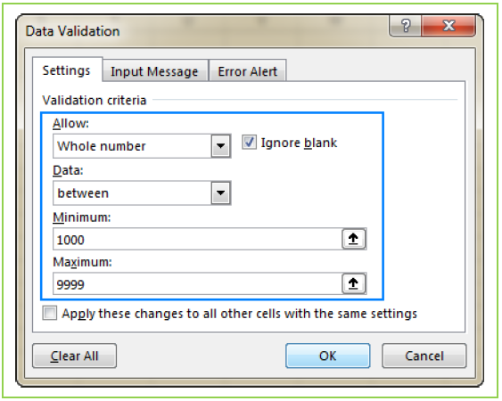
Figure 1.35 range number between 1000 to 9999
With the validation rule configured, either click OK to close the Data Validation window or switch to another tab to add an input message or/and error alert.
3. Add an input message (optional)
If you want to display a message that explains to the user what data is allowed in a given cell, open the Input Message tab and do the following:
- Make sure the Show input message when cell is selected box is checked.
- Enter the title and text of your message into the corresponding fields.
- Click OK to close the dialog window.
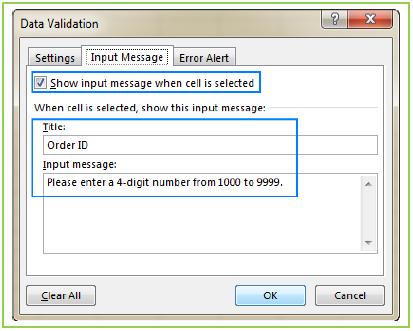
Figure 1.36 Input Message
As soon as the user selects the validated cell, the following message will show up:

4. Display an error alert (optional)
To configure a custom error message, go to the Error Alert tab and define the following parameters:
- Check the Show error alert after invalid data is entered box (usually selected by default).
- In the Style box, select the desired alert type.
- Enter the title and text of the error message into the corresponding boxes.
- Click OK.
APPLICATION ACTIVITY 1.7
1. Define the following Terms:
a. Data validation
b. Input message
c. error Alert
2. What is the benefit of validating a document?
3. Analyze the table below and Apply an input message to IdNumber
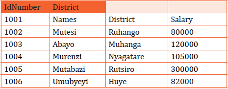
4. Validate column IdNumber so that the entered number must be between 1000 and 7777
1.5. Using other Excel templates
ACTIVITY 1.8
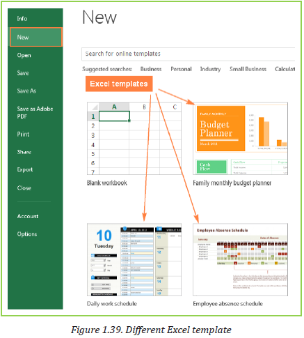
Microsoft Excel templates are a powerful part of Excel experience and a great way to save time. Excel templates can also help you create consistent and attractive documents that will impress your colleagues or supervisors.
Templates are especially valuable for frequently used document types such as Excel calendars, budget planners, invoices, inventories and dashboards.
a. Creating a workbook from an existing Excel template
Instead of starting with a blank sheet, you can quickly create a new workbook based on an Excel template. The right template can really simplify your life since it makes the most of tricky formulas, sophisticated styles and other features of Microsoft Excel that you might not be even familiar with.
To make a new workbook based on an existing Excel template, perform the following steps.
- Switch to the File tab
- Click New
Templates provided by Microsoft displayed.
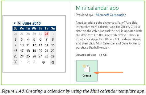
1. To preview a certain template, simply click on it. A preview of the selected template will show up along with the publisher’s name and additional details on how to use the template.
2. If you like the template’s preview, click the Create button to download it.
For example, I’ve chosen a nice mini calendar template for Excel:
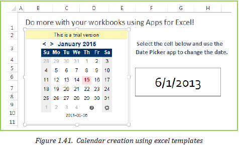
That’s it - the selected template is downloaded and a new workbook is created based on this template right away.
b. Finding more templates
To get a bigger selection of templates for your Excel, type a corresponding keyword in the search bar:
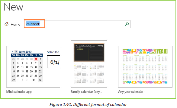
If you are looking for something specific, you can browse available Microsoft Excel templates by category. For example, see how many different calendar templates you can choose from:
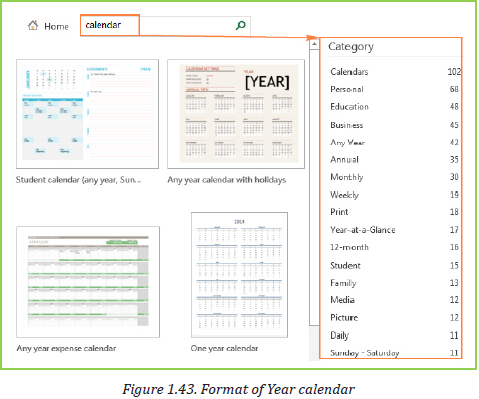
Note. When you are searching for a certain template, Microsoft Excel displays all relevant templates that are available on the Office Store.
c. Making a custom Excel template
Making your own templates in Excel is easy. You start by creating a workbook in the usual way, and the most challenging part is to make it look exactly the way you want. It is definitely worth investing some time and effort both in the design and contents, because all formatting, styles, text and graphics you use in the workbook will appear on all new workbooks based on this template.
In an Excel template, you can use save the following settings:
- The number and type of sheets
- Cell styles and formats
- Page layout and print areas for each sheet
- Hidden areas to make certain sheets, rows, columns or cells invisible
- Protected areas to prevent changes in certain cells
- Text that you want to appear in all workbooks created based on a given template, such as column labels or page headers
- Formulas, hyperlinks, charts, images and other graphics
- Excel Data validation options such as drop-down lists, validation messages or alerts, etc.
- Calculation options and window view options.
- Macros and ActiveX controls on custom forms
Note: Once you’ve created the workbook, you just need to save it as a .xlt or .xltx
file (depending on which Excel version you use) instead of usual .xls or .xlsx.
If you need the detailed steps, here you go:
- In Excel 2013, click File
- In the Save As dialogue, in the File name box, type a template name.
- Under Save as type, select Excel Template (*.xltx) if you are using Excel 2013, 2010 or 2007.In earlier Excel versions, select Excel 97-2003 Template (*.xlt).
If your workbook contains a macro, then choose Excel Macro-Enabled Template (*.xltm).
When you select one of the above template types, the file extension in the File
Name field changes to the corresponding extension.
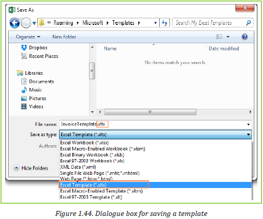
1. Click the Save button to save your newly created Excel template.
Where to download Excel templates
As you probably know, the best place to look for Excel templates is Office. com. Here you can find a great lot of free Excel templates grouped by different categories such as calendar templates, budget templates, invoices, timelines,
inventory templates, project management templates and much more.
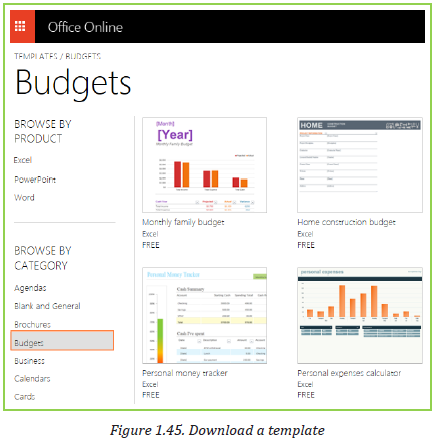
To download a particular Excel template, simply click on it. This will display a brief description of the template as well as the Open in Excel Online button.
APPLICATION ACTIVITY 1.8
1. Define the following Terms:
a. Microsoft Excel template
b. Business
c. Calendars
2. Design your personal Card using Microsoft Excel template (be specific)
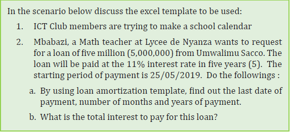
3. You want to request a loan in BK
a. Using Loan Amortization template calculate the monthly payment
b. In which year will you finish paying?
c. Calculate the total interest to pay
d. If you get more means and you want to pay one year before the end of your contractual payment how much money will you
save on unpaid interest
END UNIT ASSESSMENT