UNIT 7: THEORY OF DEMAND AND SUPPLY

Key unit competence: To be able to analyse demand and supply Conditions in the market to make right economic and entrepreneurial decisions
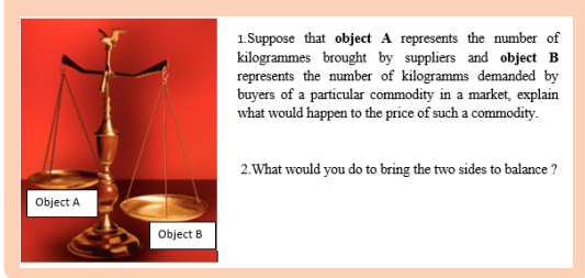
Introductory activity
Case study During scarcity of some commodities when prices are high, the government intervenes in fixing the prices so that the consumer cannot suffer from those highest prices. However, this doesn’t happen all the time when the government has adopted the mixed economy. Additionally, another intervention happens when the government needs to protect producers from closing their doors due to excess supply which results in lower prices. Under this circumstance, the government can either fix the prices you cannot go below or subsidize some goods so that the prices could be affordable.
In the past month of March to April 2022, the number of trucks carrying fuel from the Mombasa port in the Republic of Kenya into Rwanda reduced. It was said that the cause of this fuel crisis was simply the Russia-Ukraine war. At pump stations countrywide, Fuel was very expensive since it was scarce. If the government had not acted quickly to address the situation, pump fuel prices would have shoot up tremendously.
Required:
1. Based on the case given above, Discuss the effect of scarcity of fuel on:
i). The pump price of fuel.
ii). The price of commodities in the markets countrywide.
iii). The amount of goods and services that people can be able to purchase.
2. Analyse the last paragraph in the passage above and explain the ways in which the government used ‘to address the situation’
3. Identify the different commodities used in your daily life.
4. Suggest the current market prices for each commodity identified.
5. How would you react if the prices of the commodities listed above doubled?
6. Discuss and explain how the above prices are determined in a market.
7.1. Theory of demand
7.1.1. Law of Demand, Demand schedule and Demand curve
Learning activity 7.1.1
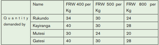
The following is the demand for sugar by Albert, Bernard, Cecile, and David at different price levels in different periods (Months) in the market of Gicumbi:
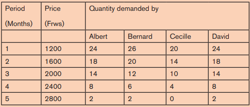
From the given data answer the following questions:
a) What is your observation about the change in prices and quantity demanded?
b) Draw a separate table for each consumer
c) On each separate table, design its demand curve to show how the given consumer responds to changes in price.
d) Using the table drawn for each consumer, derive the curve that shows how all consumers in Gicumbi market respond to changes in market prices.
e) Knowing that a curve drawn for each consumer is called « an individual demand curve, suggest an appropriate name for a curve that shows how all consumers in a market respond to change in price.
i) Meaning of key terms
– Demand is the amount of goods or services that a consumer is willing and able to purchase at various price levels per period (per day, per week, etc.)
– Effective demand/ Quantity actually demanded refers to the amount of commodity actually available and purchased at various price levels in a given period,
– Ineffective demand/Latent demand refers to the desire that is not backed by ability to buy something.
– Quantity Demanded refers to the amount of commodity the buyers are willing and able to buy at various price levels at particular time.
ii) Demand function
It is a statement of the technical relationship between quantity demanded of a commodity and those determinants of demand. ( , , , , , ,...) 1 Qdx f P P Y T S G x n− = Where: Qdx = Quantity demanded of commodity x Px =Price of commodity x Pn−1=Price of another commodity T = Tastes and preferences S = Season G = Government policy
a. Law of Demand
The law of demand states that other factors remain constant (ceteris paribus), the higher the price of a commodity, the lower the quantity demanded for that commodity and the lower the price the higher quantity demanded of that commodity.
It is commonly known that when the price changes, the demand for commodity also changes. “Ceteris paribus, When the price of a commodity increases, quantity demanded reduces
“ Ceteris Paribus: This concept is a Latin phrase or concept meaning “other factors remaining constant”. Most of the time we use it to show that the statement, law, theory or analysis stands if we assume all those factors do not interfere.
Example: The quantity demanded of a commodity will increase when its price falls, ceteris paribus.
This means:” the quantity demanded of a commodity will increase when its price falls, assuming other factors are constant “quantity demanded will decrease when its price increases or rises.
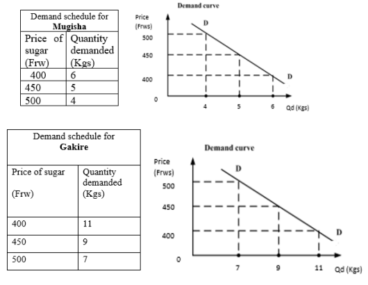
b. Demand schedule
This refers to a table that shows the various quantities of commodities that are demanded at different price levels in given period. Demand schedule can be compiled for an individual or for a group of individuals
Demand schedule is classified into:
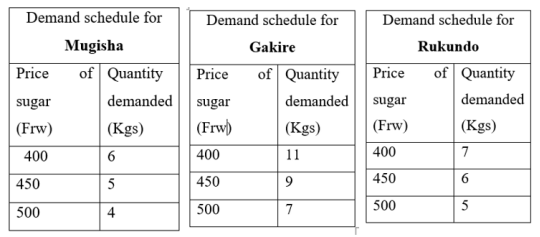
• Individual demand schedule: this refers to a table that shows the relationship between price and quantity demanded of a commodity for an individual. As the price increases, the quantity demanded reduces and vice versa, other factors remaining constant.
Example:
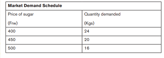
• Market demand schedule: is a table that shows the total quantities demanded by all consumers in the market at different price levels in given period.
c. Demand Curve
This is a graphical representation of the relationship between the price of a commodity and the quantity demanded of that commodity. It is the locus of points showing quantity demanded of a commodity at various price levels per period. To draw it, we plot price of commodity on the Y-axis and the quantity demanded on the X-axis. The normal demand curve slopes downwards from left to right.
The demand curve may be linear or non-linear:
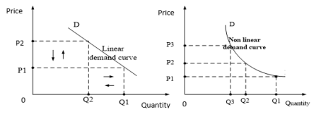
Illustrations: Demand schedule and demand curves
d. Real income effect
An increase in the price of a commodity decreases the buyer›s real income as the purchasing power of money income reduces, and a price decrease leads to an increase in real income.
e. Substitution effects
As price increases, demand falls as consumers shift their demand to relatively cheaper substitutes
Example:
When price of one commodity increases quantity demanded of that commodity reduces, and for its substitute’s commodity the price remains constant, the quantity demanded of the substitute increases.
Application activity 7.1.1
Required :
a) Construct the household demand schedule and market demand schedule using the information given in the above table.
b) Using the demand schedules in a) above, Draw the household demand curve and a market demand curve.
7.1.2. Determinants of demand
Learning activity 7.1.2
The following are the demand schedules of Shema and Kabalisa for clothes
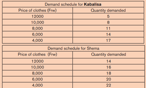
Analyze the demand schedules above and answer the questions that follow.
i) Explain why the clothing items purchased increased when prices decreased and vice versa.
ii) Why do you think Shema bought many clothes at the same price as Kabalisa
The factors that influence demand include but are not limited to the following:
i) The price of the Commodity/ good
Other factors remaining constant, when the price of a commodity falls, consumers buy more of it and vice-versa.
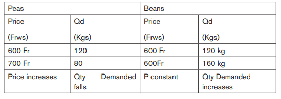
ii) Prices of other Commodities
The price of one commodity may affect quantity demanded of another commodity. The amount of a commodity demanded can be affected by changes in price levels of related commodities. Basing on their relationship we have two types of commodities:
• Substitute commodities: Substitutes are goods that serve the same purpose. When the price of one commodity increases, the demand for other increases and vice versa.
For example, when the price of Colgate increases, so does the demand for close up.
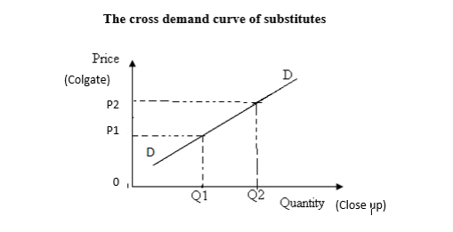
The Colgate a substitute of close up. We assume the price of close up to remain constant.
The increase in price of Colgate (substitute of close up) by P1P2 means that Colgate is more expensive than close up. The users (buyers) demand more of close up (Q1Q2) which is relatively cheaper and serves the same purpose.
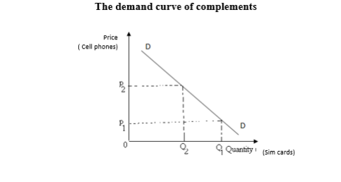
• Complementary commodities: These are goods that are used together to satisfy a need/want. e.g., Toothbrush and toothpaste, paper and pen, shoe and shoe polish, paraffin and lamp, phone and sim-card, guns and bullets, cameras and films, cars, and fuel, etc. With these commodities, one is almost useless without the other. So, when the price of one goes down, people buy more of it, and as they buy more of it, the demand for its complement increases. 130 Experimental version
E.g., When the price of cell phones reduces many people buy phones, and this increases the demand for sim cards. Or when the price of cars increases, the demand for cars reduces leading to a corresponding decrease in the demand for fuel.
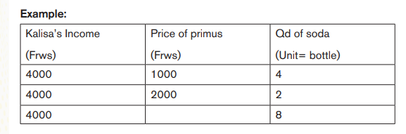
iii) Consumer’s income
A change in consumer’s income leads to a change in quantity demanded.
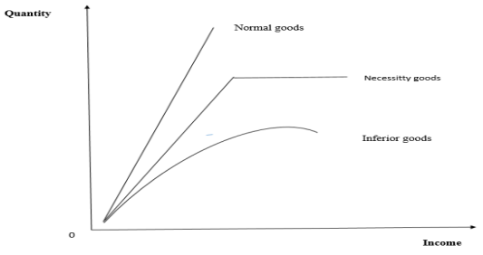
• For normal goods: An increase in consumer income leads to an increase in the quantity demanded of a normal good, while a decrease in consumer income leads to a small quantity demanded, ceteris paribus. Normal goods have a positive income elasticity of demand e.g., Sugar, Rice.
• For inferior goods: The higher the income, the lower the quantity demanded, and the lower the income, the higher the quantity demanded, ceteris paribus. Inferior goods have a negative income elasticity of demand.
• For necessity goods: Even if a consumer’s income increases, beyond a certain level the quantity demanded can no longer increase. Income elasticity of demand for normal good is zero. e.g. Salt
Income – Demand curve of Normal goods, Necessity goods and Inferior goods
iv)Government policy: such as taxation or subsidization affect the quantity demanded. For example, when taxes are increased, the quantity demanded decreases, and when taxes are decreased, the quantity demanded increases, ceteris paribus.
v) Price Expectation: When consumers expect the price of a particular good to increase in the future, they tend to buy too much of that good, which increases the quantity demanded. If they expect the price of a commodity to go down in the future, they buy less of that commodity now and reduce the quantity demanded.
vi)Seasonal Factors: When the time of the year is favorable for a commodity, the quantity demanded increases, e.g. The demand for umbrellas increases during the rainy season, the demand for Christmas cards increases during the Christmas season, etc. When the season is not favorable, the demand for this commodity decreases.
vii) Tastes and preferences: If the tastes and preferences for certain goods are favorable, the demand for that commodity will be high, and if they are unfavorable, the demand will be low. viii)Income distribution in an economy: When incomes are evenly distributed in an economy, demand for households in the economy is high, and when they are unequally distributed, demand is low.
ix)Population size: A larger population size has a higher purchasing power than a small one and thus leads to high demand and vice versa.
x) Fashion: When goods are in fashion, they are in high demand, unlike when they are obsolete or out of fashion. xi)Habit: Some commodities are consumed due to the habit for example if it is a habit for someone to consume beer, he or she will buy more of it and vice versa.
xii) Credit availability: When credit is available at low interest rates, people can access it and borrow for consumption, thereby increasing the quantities demanded and vice versa.
xiii)Money Supply: When there is no inflation, increase in money supply leads to increase of quantity demanded and decreasing the money supply decreases the quantity demanded, other factors remain constant.
xiv) Degree of advertising: A high degree of advertising attracts more customers and thus increases their quantity requirements and vice versa. This is because advertising greatly influences people’s purchasing decisions.
xv) Social, Cultural and Political Factors: Demand for most goods tends to increase during festive seasons such as Christmas, Easter, Eid, Independence. However, some social culture and political factors may result in lower demand for a commodity. For example, some cultures and religions prohibit their people from consuming some commodities, resulting in less demand for them.
xvi) Composition of population in terms of sex: If there is an increase in number of females, the demand for dresses and other females’ attire would increase and vice versa.
xvii) Education: This affects people’s tastes and preferences. Where there is a difference in people’s level of education, their levels of consumption of certain commodities differ. For example, highly educated people demand more for newspapers than uneducated people.
xviii) Income levels of neighbors: Consumers tend to consume the same goods as their neighbors. So, if neighbors have high income and a poor household would consume more goods to keep up with the rich neighbors.
xix) Age structure: When the composition of a certain population is dominated by a certain age group, demand is influenced accordingly. For instance, if most of the population are young people, demand for entertainment increases and vice versa, other factors remain constant. If there is increase in number of children, quantity demanded of toys, children’s clothing would increase.
xx) Demand level over the past period: Consumers tend to maintain the same level of demand. Thus, the higher the demand was in the past, the greater the quantity demanded in the present period. If income was low in the previous period, the quantity demanded would be low because of little or no savings to spend in the present.
Application Activity 7.1.2
The price of household goods such as kitchen utensils in Kigali markets remained constant in a certain period, but the quantity demanded doubled.
Discuss the factors that may have caused this increase in quantity demanded of the household goods.
7.2. Types of demand & Abnormal Demand Curves
Learning activity 7.2
Analyse the following sets of commodities and answer the questions that follow:
Set X: Butter and Margarine; Tea & Coffee; Colgate & White dent; Private schools and public schools.
Set Y: Cars and fuel; Shoes and Polish; pen and ink; Mobile Phones and Sim Cards; Computer Hardware and Computer Software; Toothbrush and Toothpaste.
Set Z: Land for farming or building houses; an iPhone used as camera, for internet access and making phone calls; Water for cooking, bathing, washing, mopping, drinking.
Set W: Computer and Bicycle; Mattress and Shirt; Pen and Plate; Water and Airtime
a) After analyzing the above sets, which economic term can you give to each set of commodities (Set X, Set Y, Set Z and Set W)?
b) Explain the relationship between commodities in each Set X, Y, Z and W.
c) Explain how changes in price affect demand of commodities in each set
7.2.1 Types of demand
i) Joint / Complementary demand
This is the demand for commodities that are consumed together for greater satisfaction, such that an increase in demand for one automatically leads to an increase in demand for the other commodity and vice versa. e.g., Cars and petrol, phone and SIM card, camera and films, toothpaste, and toothbrush.
ii) Competitive demand: This refers to the demand for goods that serve the same purpose (substitutes) such that an increase in demand for one lead to a decrease in demand for the other, e.g., Colgate and Close up, Beans and Peas,
iii) Derived demand: This is the demand for a commodity not for its own sake, but for the purpose for which it is used, i.e. the demand for that commodity is the direct result of the demand for a commodity that it is used to produce.
e.g.: – Demand for factors of production such as land, labor capital as a result of the demand for goods that can be produced with these factors of production.
– The government needs many economists; the economics teachers have to be recruited.
iv)Composite demand: This is the demand for a commodity that serves multiple purposes/uses such that its total demand is the sum of the quantity demand for multiple uses, e.g. Wood, Electricity, Water. For instance, the amount of water needed depends on the water needed for washing, cleaning, and drinking, mopping, …
v) independent demand: This is the demand for goods that is not affected by the demand for other goods. For example, demand for shoes is unrelated to demand for cell phone.
7.2.2. Abnormal demand curves
Abnormal curves are the curves that do not obey the law of demand. Circumstances in which abnormal demand curves arise:
i) Goods of ostentation
These are categories of goods demanded by those who want to emphasize their social and economic status by showing off what they consume. Such goods only serve their purpose if they are expensive and demand increases. the price increases, so does the demand. They are luxurious goods. The quantity demanded for these goods rises as the price rises.
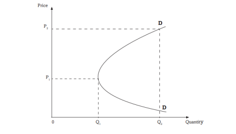
A smaller quantity OQ1 of the luxury good is bought at price OP1. With a higher price OP2, more quantity OQ2 is demanded. The demand curve for goods of ostentation is abnormal at higher prices.
ii) Price expectation
If the prices of commodities are expected to increase further in the future, the consumer will buy more of the commodities even if the current price of the goods increases. In the future, consumers will want to buy the same goods at significantly higher prices. Even though prices are expected to fall further in the coming days, consumers buy less in the current period and wait for prices to fall.
iii) Consumer’s ignorance effect on the market conditions
If consumers do not know the price, quality, packaging and labeling of the goods and other market conditions, the demand curve may be abnormal. An increase in the price of a commodity can be understood as an increase in quality that encourages the consumer to buy more of it. A consumer who is unaware of the existence of substitute goods may be forced to buy a good at a high price regardless of whether there is a cheap substitute.
iv)Depression effect
This is the time of low prices, low incomes, low purchasing power and low economic activity. During this period of low prices, the quantity demanded is also low.
v) Necessity goods
The demand for such commodities is perfectly inelastic. An example of such goods is medicine. Its demand remains high despite the increase in its price. For instance, a patient shall be willing and ready to pay any price for the subscribed medicine if he or she has the ability to pay.
vi)Case of Giffen goods
If consumers do not know the price, quality, packaging and labeling of the goods and other market conditions, the demand curve may be abnormal. An increase in the price of a commodity can be understood as an increase in quality that encourages the consumer to buy more of it. A consumer who is unaware of the existence of substitute goods may be forced to buy a good at a high price regardless of whether there is a cheap substitute.
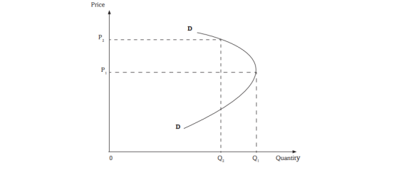
At the price OP1 the consumer buys the quantity OQ1. When the price increases to OP2, the quantity demanded decreases to OQ2. This is because as the price goes down, consumers buy less of the Giffen merchandise to be left with a little more income to purchase a different merchandise they previously could not afford. The demand curve for Giffen goods is abnormal at lower prices.
Application Activity 7.2
Analyse the factors that influence people ‘s purchasing decisions in a market.
7.3. Change in quantity demanded Vs Change in demand
Learning activity 7.3
Use the demand function to identify the factors that may influence a change in demand
a. Change in quantity demanded
This refers to the increase or decrease in the quantity of a commodity purchased in the market due to changes in price, all things being equal “Ceteris paribus”. This is illustrated by moving along the same demand curve.
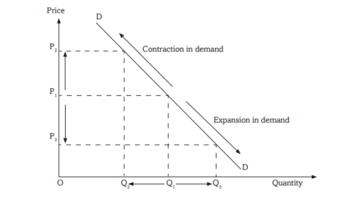
A price change from OP1 to OP2 leads to a reduction in quantity demanded from OQ1 to OQ2. The opposite is also true. Likewise, a price change from OP1 to OP3 leads to an increase in quantity demanded from OQ1 to OQ3.
All of this shows movement along the demand curve.
b) Change in Demand
Refers to an increase or decrease in demand that is caused by a change in other factors, other than price. These factors include changes in income, prices of other commodities, tastes and preferences. The change in demand is illustrated by a shift in the demand curve
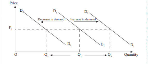
At price OP1, the quantity demanded is OQ1. Price remains constant but quantity demanded either falls to OQ2 and the demand curve also shifts to D2 or rises to OQ3 and the demand curve shifts to D3. A change in demand can be an increase in demand. In such a case, the demand curve shifts to the right. It can also be a fall in demand, where the demand curve shifts to the left
Application Activity 7.3
1. Using graphical representation, differentiate between changes in demand and changes in quantity demanded.
2. Examine the factors that may influence the change in quantity demanded
7.4. Theory of supply
7.4.1. Law of Supply, Supply Schedule, and Supply curve
Learning activity 7.4.1
The following are the supply schedules for Ishimwe, Keza, Higiro and Dukundane for sugar at different price levels during different periods (Months) in the Huye market.
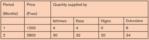
Answers the following questions using the data provided in the above table :
a) What is your observation about the change in prices and quantity supplied?
b) Draw a separate table for each supplier
c) On each separate table, design its supply curve to show how the given supplier responds to changes in price.
d) Using the table drawn for each supplier, derive the curve that shows how all suppliers in Huye market respond to changes in market prices.
e) Given that a curve drawn for each supplier is called « an individual supply curve, suggest an appropriate name for a curve that shows how all suppliers in a market respond to change in price
i) Definitions of key terms
– Supply refers to the quantity of commodity that producers are willing to offer for sale to the market over a given period at a given price.
– Quantity supplied
This refers to the quantity of a commodity that producers are willing and able to bring to market at different prices per period. The amount delivered is a desired flow. It measures how much the grower wants to sell and not how much they actually sell.
Note that the quantity supplied may differ from the quantity produced, as some of the goods produced may not be delivered to the market.
ii) Supply function
Supply function shows the technical relationship between quantity supplied and the main determinants of quantity
supplied.
a. Law of Supply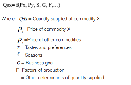
This law states that, “ceteris paribus”, the higher the price, the higher the quantity supplied and vice versa. There is a positive relationship between price of a commodity and quantity supplied of that commodity. Ceteris paribus when the prices are increasing, the producers supply more, and when the prices are falling, they supply less.
b. Supply Schedule
A delivery schedule is a table that shows different quantities of a commodity that a producer can supply at different prices per period.
Example:
A supply schedule may be individual supply schedule (for a single producer or seller) or a market supply schedule. .Individual supply schedule is a table showing the quantities supplied by a single seller/producer at different price levels
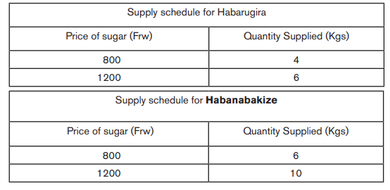
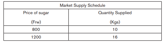
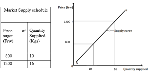
• Market supply schedule is a table showing the sum of all individual producer/seller quantities in the market for a given commodity at different prices levels in a given period. various quantities of a commodity that all the producers/sellers are willing to sell at various levels of price, during a given time.
c. Supply curves
The supply curve is a locus of points that shows the quantity of a product brought to the market at different prices per period. Normally, the supply curve goes up from left to right, showing that the higher the price, the higher the quantity supplied, other factors remaining constant.
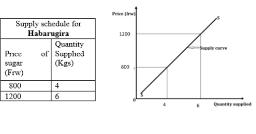
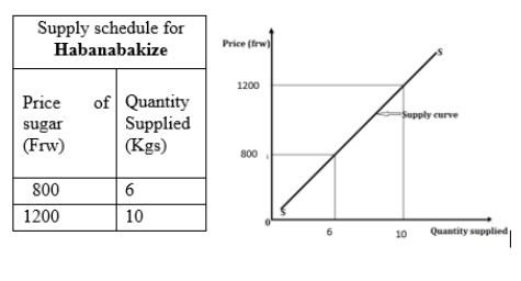
Individual supply curve
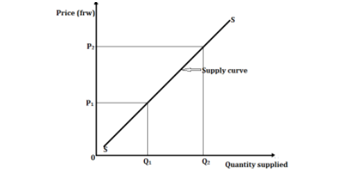
The supply curve is sloping, showing that as the price increases from OP1 to OP2, the quantity supplied also increases from OQ1 to OQ2. This clarifies what the law states. The supply curve may not go through the origin since suppliers usually have a floor (reserve) price below which they will not deliver or sell. For example, the minimum price in the curve above is P1. The quantity therefore remains at zero until this minimum price is reached.
Individual supply curves:
Market supply curve
Application Activity 7.4.1
The following are the supply schedules of Uwase and Kalisa for sugar
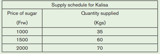
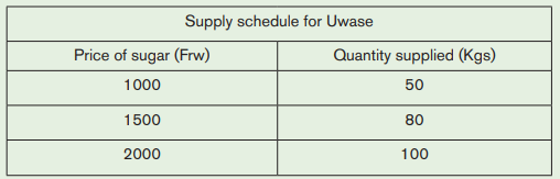
Analyse the supply schedules above and answer the questions that follow. Explain why the quantity of sugar sold increased when prices increased and vice versa.
7.4.2. Determinants of Supply
Learning activity 7.4.2
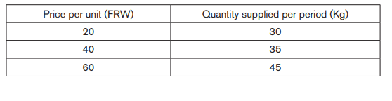
The following are the Supply schedules of selling sweet potatoes for Umulisa and Kabatesi
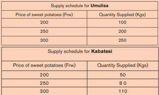
The following are the Supply schedules of selling sweet potatoes for Umulisa and Kabatesi Analyse the Supply schedules above and answer the questions that follow
i) Explain why the quantity sold increased when prices increased and vice versa.
ii) Apart from price changes, what do you think would make Umulisa and Kabatesi did not sell the same units of sweet potatoes?
i) The price of the commodity itself:
Other factors remaining constant, the higher the price, the higher the quantity supplied of a commodity and the lower the price, the lower the quantity supplied of that commodity.
ii) The price of other commodities. If the prices of competing goods increase, it becomes more profitable to produce those competing goods, which are more profitable. When the prices of competing goods fall, the quantity of a goods supplied increases because it becomes more profitable to produce the goods whose price is relatively higher ceteris paribus.
iii) Number of Firms or Producers:
The more producers involved in the production of a given commodity, the more of that commodity will be supplied, and if there are few producers, the quantity of that commodity supplied will be small.
iv)Goals a firm:
If the goal of the firm is to maximize sales, more will be supplied and if it is to maximize profit, less will be supplied.
v) Cost of production:
The lower the cost of production, the higher the quantity supplied and vice versa.
vi)The level of technology: The more advanced the technology, the higher the quantity supplied and the less advanced the technology, the smaller the quantity supplied.
vii) Demand for the commodity:
There is a direct relationship between the demand for a commodity and its supply. i.e., an increase in demand for a commodity makes it more profitable as this increases its price. Thus, an increase in demand encourages producers to produce more output to meet the available demand. On the other hand, a drop in demand for a commodity hampers its production and supply.
viii)Government policy:
When the government imposes high taxes on producers, production and supply decrease, and when the government subsidizes producers, production and supply increase.
ix)Seasonal Factors: When the season is favorable for a particular commodity, the supply will be high, and when the season is not favorable, the quantity supplied will be low.
x) Degree of freedom of entry of new firms into production: Some industries have entry barriers in the form of start-up costs, patents, technology, price limitation by the already existing company. When entry of new firms into the industry is free, supply increases, while restricted entry of new firms keeps supply down.
xi)Time: Supply is high in the long term and low in the short term. It is very easy for producers to supply more of a commodity over a long period of time, and they can only produce less of that commodity in a short period of time.
xii) Population/market size: The larger the population, the larger the market size, i.e., the higher the quantity offered and vice versa, other factors remain constant.
xiii)Expectation of future price: If sellers expect the price to rise in future period, they sell little in current period and the supply curve shifts to the left. If sellers anticipate the price will fall, they try to sell more in current period, the supply shifts to the right.
xiv) Gestation period: This is the length of time between when the decision is made to produce and supply a good and when the output is actually produced and supplied. A long gestation period reduces the supply in the current period. A short gestation period increases the supply in the current period.
xv) Political climate:
The stability in the country will encourage investment, production and supply of goods and services, while instability and insecurity in the country will discourage investment, production and supply of goods and services.
xvi) Climate and weather: When the climate/weather is favorable for production, production and supply will be high, especially in the agricultural sector, and vice versa than when the climate is unfavorable. This climate includes natural factors such as drought, rain, wind, sunshine, etc.
Application Activity 7.4.2
Assume the prices of maize flour in your home locality remained constant over a period of time but the quantity supplied doubled. Discuss the factors that may have contributed to the increase in quantity of maize flour supplied.
7.4.3. Types of Supply & Abnormal Supply Curves
Learning activity 7.4.3
Given commodities grouped in the following manner: Group one Yoghurt and Cheese, Banana juice and Urwagwa (banana wine) Group two Beef and hides (skins), diesel and petrol
a) Economically, how would you name the above category of goods as grouped in Group one &Group-two?
b) Explain the relationship between commodities in each group
c) Explain how price changes affect the supply of commodities in each category of goods Group one and Group two ).
a. Types of Supply
i) Competitive supply: This is the supply of two goods that use the same resources, so increasing the production and supply of one product decreases the resources available for the production and supply of another.
ii) Joint supply: This is the supply of two goods produced together such that an increase in the supply of one product results in an increase in the supply of another, e.g., the offer of beef and skins.
b. Abnormal supply curves
Abnormal supply curves/Regressive curves are the supply curves that violate the law of supply.
Such curves appear under the following conditions:
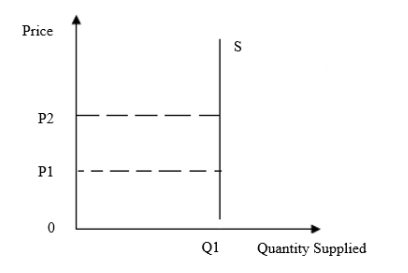
i) Fixed supply in the short run:
If there is not enough time available to allow the producer to organize and increase production and supply, the quantity supplied can remain constant despite the increase in the price of the goods. For this case, the curve can look like as follows:
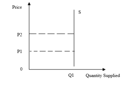
ii) The supply of land:
Land as a factor of production refers to all resources above, on, and under the surface of the earth that are used in the production process. It has fixed supply i.e.; the size of land does not change. Its supply curve is perfectly inelastic as shown in the following curve:
iii) Backward-bending labour supply curve
Backward-bending labour supply curve is a graphical illustration showing a situation in which as real wages increase beyond a certain level, people will substitute leisure for paid work time and so higher wages lead to a decrease in the labour supply. The supply curve behaves normally at low wages and becomes abnormal at higher wages.
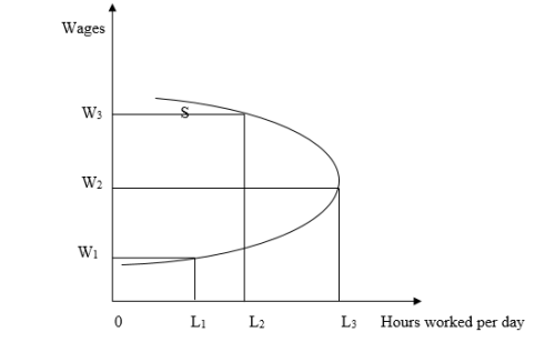
The supply of labor increases from OL1 to OL2 when the wage is increased from OW1 to OW2, beyond wage OW2, labor supply reduces to OL3 when the wage is increased to OW3. This creates a backward bending supply curve of labor.
The supply curve of labor bends backwards when wages are increased because of the following reasons:
– Increase in wages stimulates a strong preference for leisure to work. At higher wages, workers tend to like more of leisure than work, so they work for fewer hours.
– Presence of target workers. When wages are increased, workers reach their target quickly and start working fewer hours after reaching their target.
– If there is an insecurity in the area where the workplace is located, this threatens the employees, who can reduce their working hours regardless of the wage increase.
Application Activity 7.4.3
Analyse the reasons why people supply goods to the market.
7.4.4. Change in Supply Vs Change in quantity supplied
Learning activity 7.4.4
Given the supply function, what do you think is the difference between change in supply and
change in quantity supplied.
a. Change in quantity supplied
This refers to the change in the quantity of goods available for sale on the market at any given time due to a change in he price of that commodity, other factors remaining constant. A change in quantity supplied is represented by movement along the same supply curve.
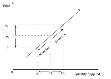
An increase in price from 0P1 to 0P3 leads to an increase in quantity supplied from 0Q1 to 0Q3 and decrease of price from 0P1 to 0P2 leads to a decrease in quantity supplied from 0Q1 to 0Q3 , ceteris paribus.
i) Increase in quantity supplied (Extension of supply curve)
This is an increase in the quantity of commodities available for sale over a given period. When the price of the commodities increases, ceteris paribus, increase in quantity supplied is illustrated by moving upwards along the same supply curve.
ii) Decrease in quantity supplied (Contraction of supply curve)
This is a reduction in the quantity of commodities available for sale over a period. When The price of commodities falls, other factors remain constant, increase in quantity supplied is illustrated by moving downwards along the same supply curve.
b. Change in Supply
This refers to an increase or decrease in the amount of a commodity supplied in the market at a particular time due to other determinants of supply at a constant price. This increase or a decrease of quantity supplied is illustrated by a shift movement of supply curve.
i) Increase in supply (Shift of supply curve to the right)
This refers to an increase in the amount of goods offered to the market for sale at a given time at constant price due to other favorable conditions of supply leading it to shift to the right.
Graphical Illustration
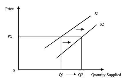
At constant price 0P1, quantity supplied is 0Q1. Due to changes in other factors that influence the supply, quantity supplied increases from 0Q1 to 0Q2 at constant price(0P1).
An increase in supply of a commodity may be brought about by an increase in the number of producers, price of competing commodities, improvement in technology, entry of new firms into the industry, favorable natural factors, increase in demand for the commodity, change in goals of the firm, decrease in prices of factors of production, etc.
ii) Decrease in supply (shift of supply curve to the left)
This refers to a reduction in the amount of goods offered to the market for sale at a given time at constant price due to other unfavorable conditions of supply leading a shift of the supply curve to the left.
Graphical Illustration
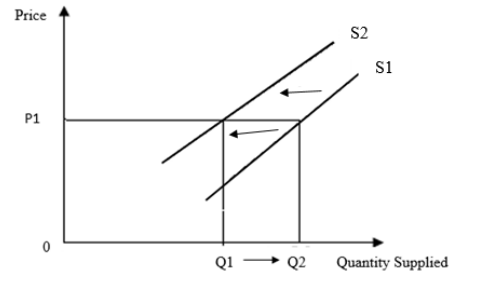
A decrease in the supply of a commodity may be a result of a decrease in the number of producers, decline in technology, exit of some firms from the industry, increase in costs of production due to increase in taxes of producers, unfavorable natural factors, decline in demand for the commodity, change in goals of the firm, increase in prices of factors of production, increase in the price of a competing commodity, etc.
Application Activity 7.4.4
Using graphical illustrations, show the difference between change in supply and change in quantity supplied
7.5. Equilibrium price and quantity supplied
Learning activity 7.5.
7.5.1. Definitions of key terms
Equilibrium refers to the situation of stability when the forces as they exist at particular time have no tendency to change. For example, equilibrium in the market is attained when the quantity demanded equals quantity supplied.
An economy is in general equilibrium when all sectors are stable, i.e., quantity of goods supplied equals quantity of goods demanded, money provided by savers equals money demanded by borrowers, labor supplied equals labor demanded, and foreign exchange earned equals foreign exchange spent.
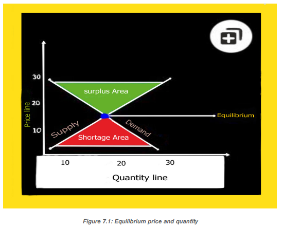
The equilibrium price is the price that prevails in the market when the quantity supplied equals the quantity demanded. At this price, the quantity of goods placed on the market by the suppliers is fully purchased by the buyers i.e. there is no surplus or shortage of commodities in the market.
Equilibrium price and quantity occur when quantity demanded is equal to quantity supplied.
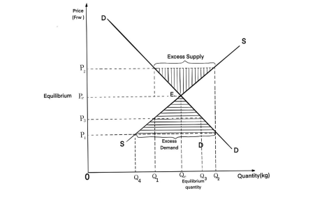
However, there could be a disequilibrium. Disequilibrium may be either a shortage (excess demand) or surplus (excess supply). When quantity demanded is greater than quantity supplied, then, there is a shortage of commodities in the market. A shortage of commodities in the market implies that buyers will compete for the available few commodities. This scenario leads to an excess demand. They will be ready to pay a high price. This excess demand will lead to price increase.
When the quantity supplied is greater than quantity demanded, there is a surplus of commodities in the market. In the figure below, quantity demanded is Q1 while quantity supplied is Q2 at price P2. Suppliers have a lot of commodities to sell. Buyers are ready to purchase less quantities compared to what the sellers have to offer. This scenario leads to an excess supply. This excess supply of commodities will force the price to go down. Suppliers will be ready to reduce the price of their commodities so that they can attract buyers.
In the long – run, once excess demand and excess supply have been dealt with, the market will remain in a state of equilibrium.
Graphical illustration
7.5.2. Calculation of equilibrium quantity and equilibrium price
Consider the following economic functions to determine equilibrium quantity and equilibrium price.
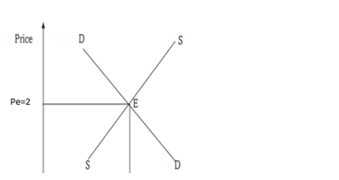
Demand function: Qd =16-3P and Supply function: Qs =6+2P Solution: Recall that Equilibrium price and quantity occur when quantity demanded is equal to quantity supplied (Qd=Qs), therefore: 16-3p=6+2p 16-6-3p+3p=2p+3p 10/5= 5p/5 P=2 At equilibrium, the price will be 2. The price already calculated is substituted in either one of the equations to find equilibrium quantity. Qd=Qs Recall: Qd=16-3P and Qs=6+2P
Qd=16-3 (2) or Qs = 6+2 (2) Qd=16-6 or Qs = 6+4 Qd=10 or Qs=10 That is to say Qe=10 and Pe=2 Where Qe = Equilibrium Quantity and Pe = Equilibrium price
Application Activity 7.5
When the price of sugar in Kimironko Market was FRW 2000, the quantity demanded was190 kg and the quantity supplied was 130 kg. A few days later, the price increased by FRW 100, and the quantity demanded decreased by 6 kg, while the quantity supplied increased by 54 kg. again, the price rose up to FRW 2,200 and the quantity demanded decreased to 170Kg while the supply increased to 200 kg.
Based on the information given, determine the equilibrium price and quantity supplied using a graphical representation.
End of unit 7 assessment
1. Describe the different factors that determine your levels of demand for the commodities you normally purchase.
2. Analyze the factors that might make someone supply much or less in a market
3. Suppose that the demand for sugar is given by the following equation, Qd =16–2P; where Qd is the amount of sugar that consumers want to buy (i.e., quantity demanded), and P is the price of sugar. Suppose the supply of sugar is Qs =2+5P; where Qs is the amount of sugar that producers will supply (i.e., quantity supplied).and P is the price of sugar. Determine the equilibrium quantity and price.