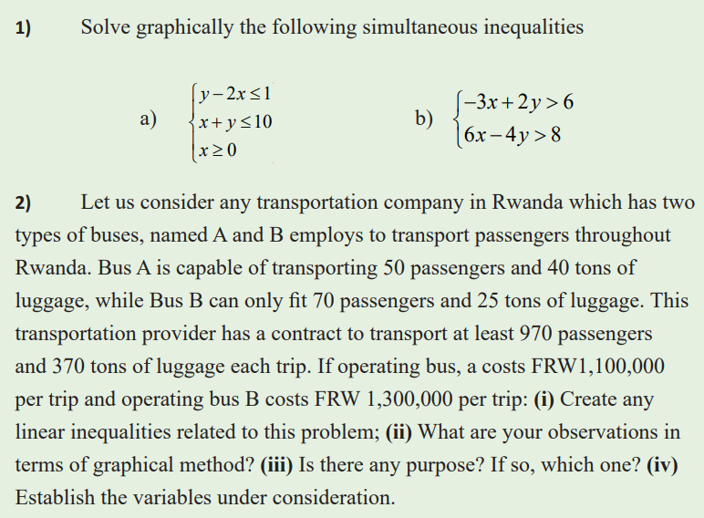
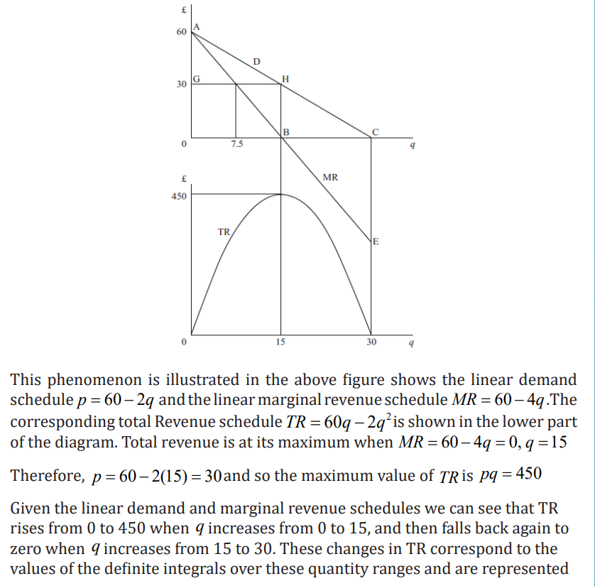
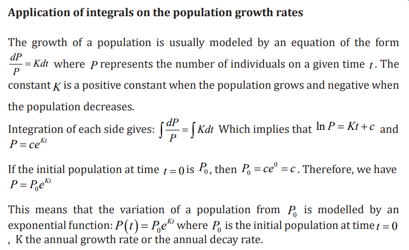
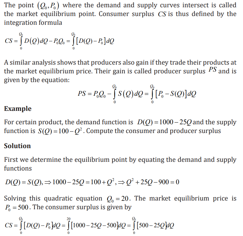
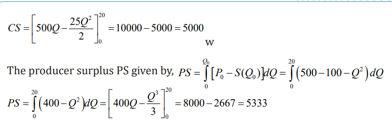
Topic outline
UNIT 1: APPLICATIONS OF MATRICES AND DETERMINANTS
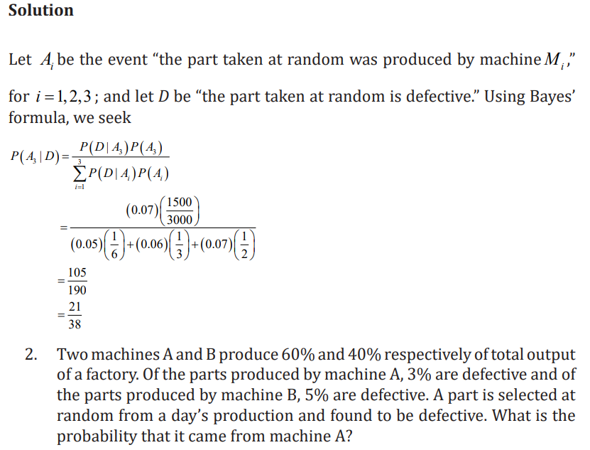
Key unit competence: Apply matrices and determinants concepts in solvinginputs & outputs model and related problems.
Introductory activity
Prices of the three commodities A,B and C are X,Y and Z per units
respectively. A person P purchases 4 units of B and sells two units of A and
5 units of C. Person Q purchases 2 units of C and sells 3 units of A and one
unit of B. Person R purchases one unit of A and sells 3 units of B and one
unit of C. in the process P, Q and R earn 15000Frw, 1000Frw and 4000Frw
respectively. Use matrix inversion to calculate the prices per unit of A, B andC.
1.1 Application of matrices
1.1.1 Economic applications
Learning activity 1.1.1
Three customers purchased biscuits of different types P, Q and R. The first
customer purchased 10 packets of type P, 7 packets of type Q and 3 packets
of type R. Second customer purchased 4 packets of type P, 8 packets of type
Q and 10 packets of type R. The third customer purchased 4 packets of
type P, 7 packets of type Q and 8 packets of type R. If type P costs 4000Frw,
type Q costs 5000Frw and type R costs 6000Frw each, then using matrixoperation, find the amount of money spent by these customers individually.
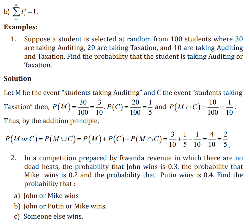
Economics is the study of shortage and how it impacts the use of resources,
the production of products and services, the growth of production and welfare
through time, as well as a wide range of other complicated issues that are of
the utmost importance to society in order to satisfy human needs and wants.
To understand money, jobs, prices, monopolies, and how the world works
on a daily basis, one must study economics. All across the world, matrices’
properties, determinants, and inverse matrices, together with their addition,
subtraction, and multiplication operations, are employed to address these real-
world issues. In economics, matrices are typically also used in the productionprocess.
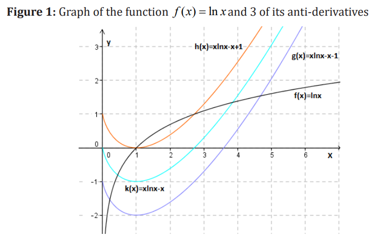
Example 1
A firm produces three products A, B and C requiring the mix of three materials
P, Q and R. The requirement (per unit) of each product for each material is asfollows.
Using matrix notation, find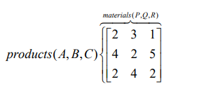
i. The total requirement of each material if the firm produces 100 units ofeach product
ii. The per unit cost of production of each product if the per unit cost ofmaterials P,Q and R is 5000Frw, 10000Frw and 5000Frw respectively
iii. The total cost of production if the firm produces 200 units of each product
Solution
i. The total requirement of each material if the firm produces 100 units
of each product can be calculated using the matrix multiplication givenbelow
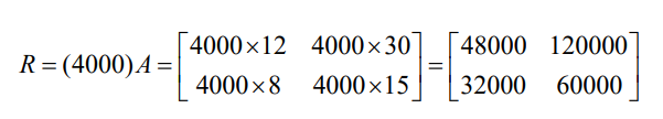
With the help of matrix multiplication, the per unit cost of production of each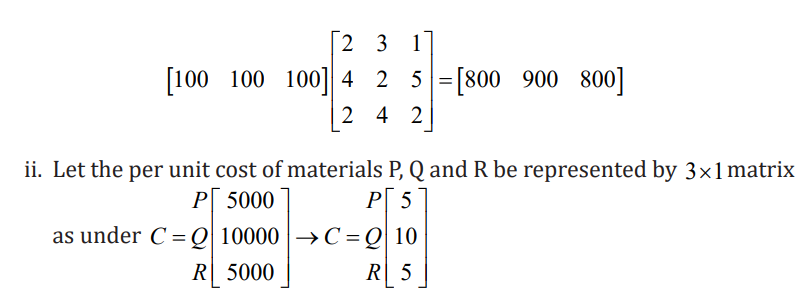
product would be calculated as
iii. The total cost of production if the firm produces 200 units of each product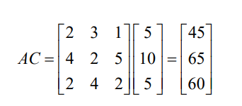
would be given as
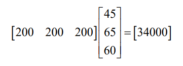
Hence, the total cost of production will be 34000Frw
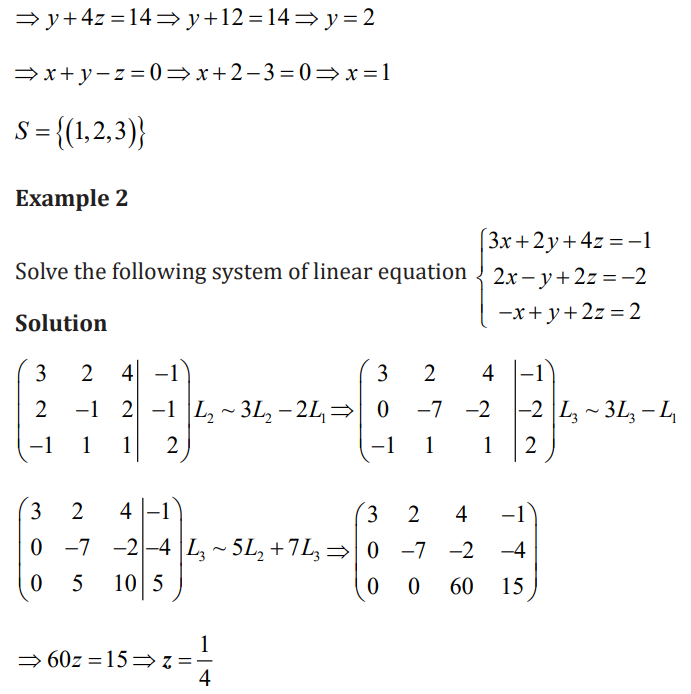
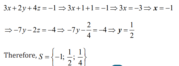
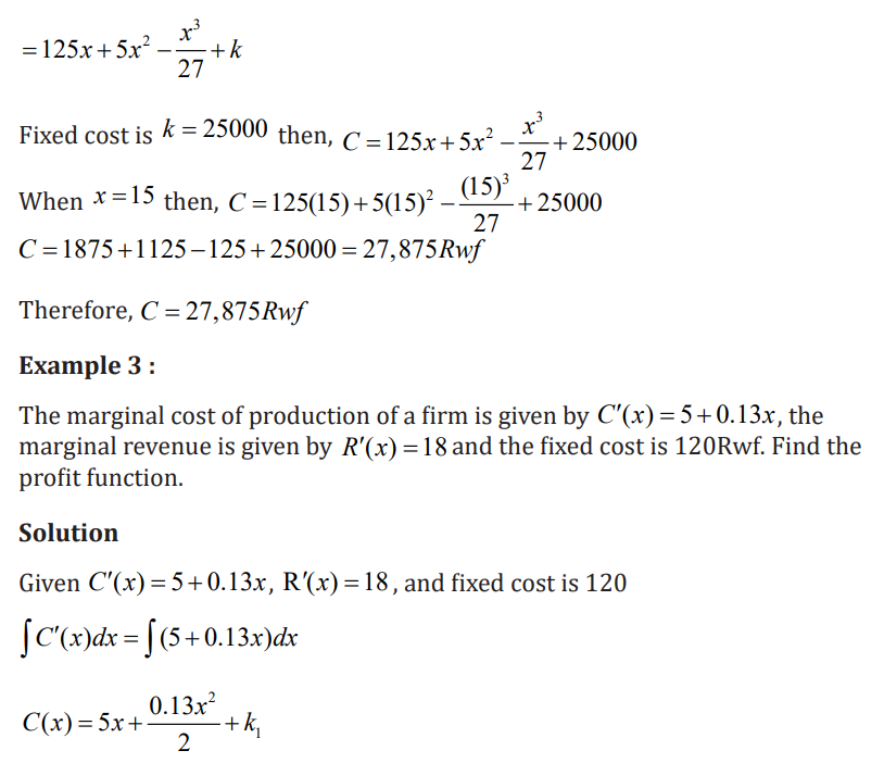
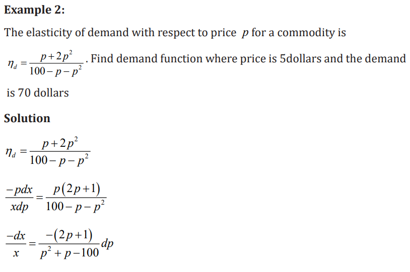
Example 2
The number of units of a product sold by a retailer for the last 2 weeks areshown in matrix a below, where the columns represent weeks and the rows
item sells for 4000Frw, derive a matrix for total sales revenue for this retailer
for these two shop units over this two-week period.
Solution:
Total revenue is calculated by multiplying each element in matrix of sales
quantities A by the scalar value 4000, the price that each unit is sold at. Thustotal revenue can be represented in Frw by the matrix
Example 3
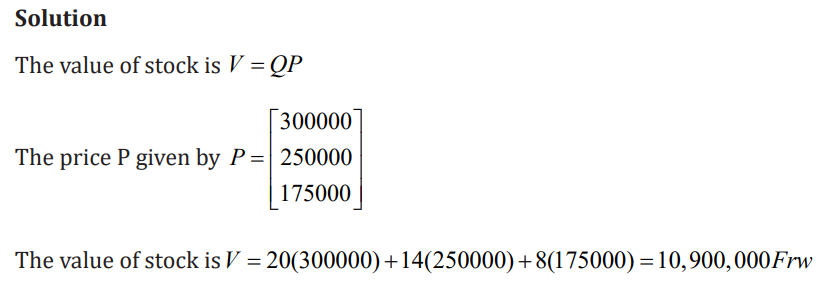
If the price of TV is 300000Frw, the price of a stereo is 250000Frw, the price of
a tape deck is 175000Frw. Present price P in a 3 1× matrix then determine thevalue of stock for the outlet given by Q = [20 14 8]
Example 4
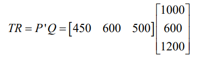
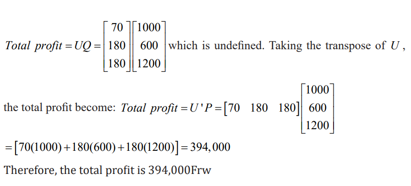
A hamburger chain sells 1000 hamburgers, 600 cheeseburgers, and 1200 milk
shakers in a week. The price of a hamburger is 450Frw, a cheeseburger 600Frw
and a milk shake 500Frw. The cost to the chain of a hamburger is 380Frw, a
cheeseburger 420Frw, and a milk shake 320Frw. Find the firm’s profit for theweek, using
a) total conceptsb) per-unit analysis to prove that matrix multiplication is distributive
Solution
a) The quantity of goods sold (Q), the selling price of the goods (P), and thecost of goods (C) can all be presented in matrix form.
Which is not defined as given. Taking the transpose of P or Q will render the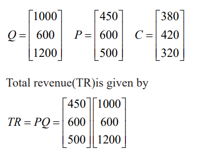
vectors conformable for multiplication. Note that the order of multiplication isimportant. Thus, taking the transpose of P and premultiplying, we get,
Application activity 1.1.1
A firm produces two goods in a pure competition, and has a following total
1.1.2. Financial applications
Learning activity 1.1.2
With clear example discuss the importance of matrices in finance andaccounting.
The process of raising cash or funds for any kind of expense is called financing. To
further handle this process, matrices are more useful in financial applications.
Matrix algebra is used in financial calculations due to the large amount of data
involved. These include managing financial risk, presenting investment orbusiness expense results or returns, and calculating value-at-risk.
To facilitate a better understanding of accounting procedures based on the
principle of double entry, various methods of solving a given problem exist. It
is very crucial to emphasize the use of matrix algebra in financial records for
accountants, bankers, and accounting students in order to prepare them foremerging trends in the business/financial world.
Application of Matrix Additive to Financial Records
In the application of matrix addition concept, one needs to examine thoroughly
the accounting records to obtain the relevant figures expressed in monetary
terms to form the required matrices. The principle of double entry in accounting
provided the need to record any business transaction twice (i.e. as debit and
credit). Accounting records in books are strictly governed by the principle
of double entry, making it easier to obtain matrices of financial transactions
from one period to the next. As a result, using appropriate matrix concepts, the
opening and closing balances can be determined from period to period with
little difficulty.
In addition, financial economics and financial econometrics rely on the use of
matrix algebra because of the need to manipulate large data inputs. Therefore,
matrix used in financial risk management, used to describe the outcomes orpayoff of an investment, and used to calculate value at risk.
Example
A finance company has offices located in province, district and cells. Assume
that there are 5 provinces, 30 districts and 200 sectors to be considered by thecompany. The workers at every level are given in the matrix form,
column stands for head clerks , and the 3rd column stands for cashiers. The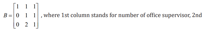
basic monthly salaries (in FRW) are as follows:
Office supervisor: 150,000
Head clerk: 120,000
Cashier: 117,500
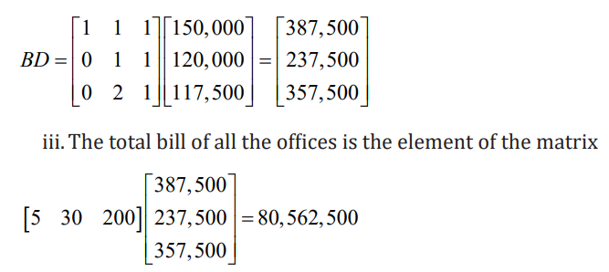
Using matrix notation, find
i. The total number of posts of each kind in all the offices taken together
ii. The total basic monthly salary bill of each kind of office and,iii. The total basic monthly salary bill of all the offices taken together
ii. Total basic monthly salary bill of each kind of offices is the elements of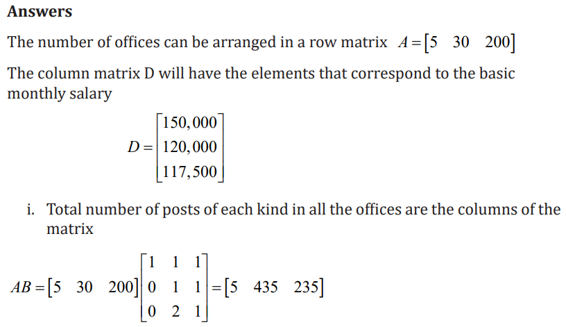
matrix
Application activity 1.1.2
Visit the finance office and look at how he/she completes the cash booksthen perform the following:
a) Create a matrix from debited and credit transactionsb) Find out transaction vector from these matrices
1.2. System of linear equations
1.2.1 Introduction to linear systems
Learning activity 1.2.1


By simplifying the second equation and found that x+ y = 3 is contradictory to
the first equation x +y = 4
A system of linear equations that has no solution is said to be inconsistent. If
there is at least one solution it is called consistent. Therefore, every system of
linear equations has either no solution, exactly one solution or infinitely manysolutions.
An arbitrary system of m equations and n variables ( m n × linear system) canbe written as

Application activity 1.2.1
Solve the following system of linear equations

1.2.2 Application of system of linear equations
Learning activity 1.2.2
A factory produces three types of the ideal food processor. Each type X
model processor requires 30 minutes of juice processing, 40 minutes of
bread processing, and 30 minutes of yoghurt processing, while each type Y
model processor requires 20 minutes of juice processing, 50 minutes of bread
processing, and 30 minutes of yoghurt processing. Each type Z model processor
requires 30 minutes of juice processing, 30 minutes of bread processing, and
20 minutes of yoghurt processing. How many of each type will be produced if
2500 minutes of juice processing, 3500 minutes of bread processing, and 2400minutes of yoghurt processing are used in one day?
When there is more than one unknown and enough information to set up
equations in those unknowns, systems of linear equations are used to solve such
applications. In general, we need enough information to set up n equations
in n unknowns if there are n unknowns. Solving such system means finding
values for the unknown variables which satisfy all the equations at the same
time . Even though other methods for solving systems of linear equations exist
, one method like the use matrices is the more important choice in economics,finance, and accounting for solving systems of linear equations.
Consider any given situation that represents a system of linear equations,consider the following keys points while solving the problem:
i. Identify unknown quantities in a problem represent them with variables
ii. Write system of equations which models the problem’s conditions
iii. Deduce matrices from the systemiv. Solve for unknown variables
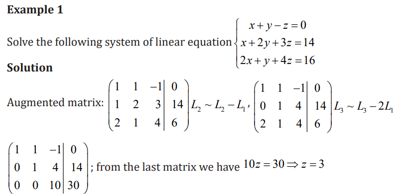
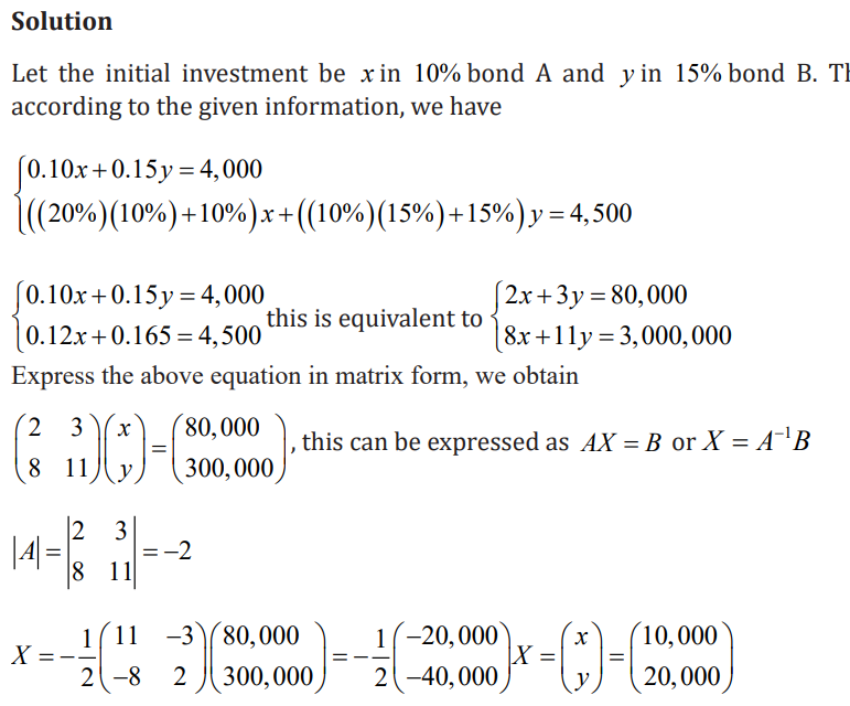
Example 1
Mr. John invested a part of his investment in 10% bond A and a part in 15% bond
B. His interest income during the first year is 4,000Frw. If he invests 20% more
in 10% bond A and 10% more in 15% bond B, his income during the second
year increases by 500Frw. Find his initial investment in bonds A and B usingmatrix method.
Hence, the production levels of the products are given by First product has 11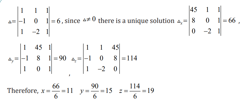
tons, second product has 15 tons and the third product has 19 tons
Application activity 1.2.2
A couple of two person has 60,000,000Frw to invest. They wish to earn an
average of 5,000,000 per year on the investment over a 5 year period. Based
on the yearly average return on mutual funds for 5 years ending december,
2022, they are considering the following funds: Personal savings at 5%,bank loans at 6%,
a) As their financial advisor, prepare a table showing the various ways
the couple can achieve their goalb) Comment on the various possibilities and the overall plan
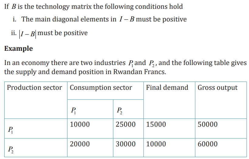
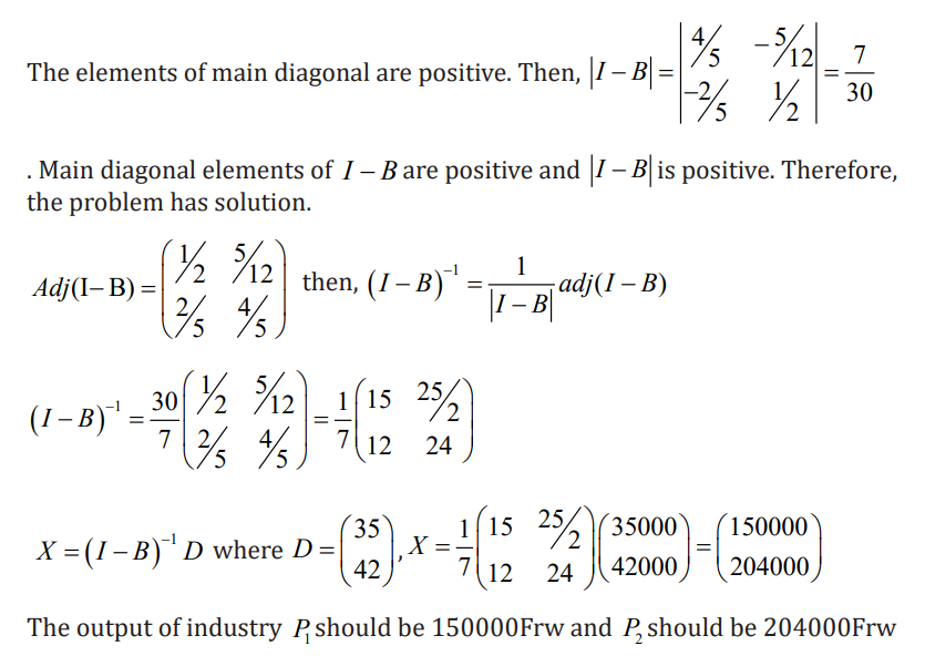
1.3. Input-outputs models and Leontief theorem for matrix oforder 2.
1.3.1 Input-outputs models ( n = 2 )
Learning activity 1.3.1
1. Generate input-output model formula and conditions hold fortechnology matrix
2. Two commodities A and B are produced such that 0.4 tons of A and
0.7 tons of B are required to produce a tons of A. similarly 0.1 tons of
A and 0.7 tons of B are needed to produce a tons of B.i. Write down a technology matrix
ii. If 6.8 tons of A and 10.2 tons of B are required, find the grossproduction of both them.
Input Output analysis is a type of economic analysis that focuses on the
interdependence of economic sectors. The method is most commonly used to
estimate the effects of positive and negative economic shocks and to analyze
the unforeseen consequences across an economy. Input-output tables are the
foundation of input-output analysis. Such tables contain a series of rows and
columns of data that quantify the supply chain for various economic sectors.
The industries are listed at the top of each row and column. The information in
each column corresponds to the level of inputs used in the production function
of that industry. The column for auto manufacturing, for example, displays
the resources required to construct automobiles (i.e., requirement of steel,
aluminum, plastic, electronic etc,). Input – Output models typically includes
separate tables showing the amount of required per unit of investment orproduction.
The use of Input-Output Models
Input-output models are used to calculate the total economic impact of a
change in industry output or demand for one or more commodities. These
models employ known information about inter-industry relationships to track
all changes in the output of supplier industries required to support an initial
increase in an industry’s output or an increase in commodity expenditures. Themodel is commonly shocked during this process.
Let us consider a simple economic model with two industries, A1 and A2, each
producing a single type of product. Assume that each industry consumes a
portion of its own output and the remainder from the other industry in order
to function. As a result, the industries are interdependent. Also, assume that
whatever is produced is consumed. That is, each industry’s total output must
be sufficient to meet its own demand, the demand of the other industry, and the
external demand (final demand).The main goal is to determine the output levels
of each of the two industries in order to meet a change in final demand, based
on knowledge of the two industries’ current outputs, under the assumptionthat the economy’s structure does not change.


Application activity 1.3.1
An economy produces only coal and steel. These to commodities serve as
intermediate inputs in each other’s production. 0.4 tons of steel and 0.7 tons
of coal are needed to produce a ton of steel. Similarly, 0.1 tons of steel and 0.6
tons of coal are required to produce a ton of coal. No capital inputs are needed.
Do you think that the system is viable? The 2 and 5 labor days are required to
produce a ton of coal and steel respectively. If economy needs 100 tons of coal
and 50 tons of steel, calculate the gross output of the two commodities and thetotal labor days required.
1.3.2 Leontief theorem for matrix of order two
Learning activity 1.3.2
1. Differentiate open Leontief Model from closed Leontief Model
2. The following are two firms that are producing units in tons foragriculture and manufacturing.
Assume that the external demand of agriculture is 80 and the one of manufacturing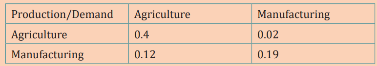
is 200. Determine the units to be produced by agriculture and manufacturingfirms in order to satisfy their own external demands.
The Leontief model is an economic model for an entire country or region. In
this model, n industries produce a numbern of different products such that
the input equals the output, or consumption equals production. It distinguishesbetween closed and open model.
The open Leontief Model is a simplified economic model of a society in which
consumption equals production, or input equals output. Internal Consumption
(or internal demand) is defined as the amount of production consumed within
industries, whereas External Demand is the amount used outside of industries.
In addition, some production consumed internally by industries, rest consumed
by external bodies. This model allows us to calculate how much production is
required in each industry to meet total demand. To determine the productionlevel, first create a consumption matrix C.
Therefore, an industry is profitable if the corresponding column in C has sum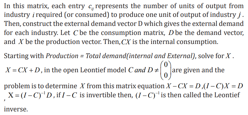
less than one.
Example
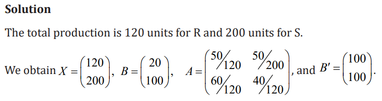
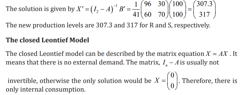
An economy has the two industries R and S. The current consumption is givenby the table
Assume the new external demand is 100 units of R and 100 units of S. Determine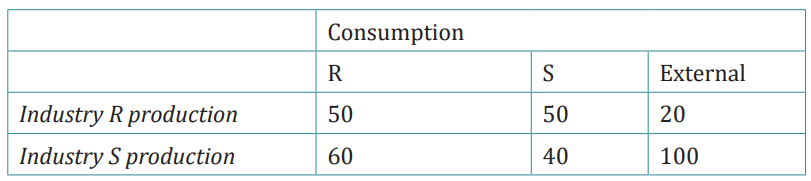
the new production levels.
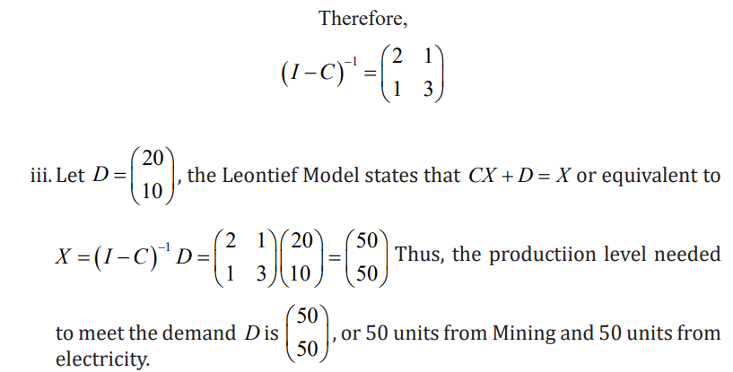
Example
Suppose that an economy has two sectors, Mining and electricity. For each
unit of output, Mining requires 0.4 unites of its own production and 0.2 units
of electricity. Moreover, for each unit output, electricity requires 0.2 units ofMining and 0.6 units of its own production.
i. Determine the consumption matrix C for this economy
ii. Find the inverse
iii. Using the Leontief model, determine the production levels from each
sector that are necessary to satisfy a final demand of 20 units from miningand 10 units from electricity.

Application activity 1.3.2
An economy has two sectors namely electricity and services. For each unit
of output, electricity requires 0.5 units from its own sector and 0.4 units
from services. Services require 0.5 units from electricity and 0.2 from itsown sector to produce one unit of services.
i. Determine the consumption matrix C
ii. State the Leontief input-output equation relating C to the productionX and final demand D
iii. Use an inverse matrix to determine the production necessary to
satisfy a final demand of 1000 units of electricity and 2000 units ofservices.
1.4 End unit assessment

Determine the number of cars of each type which can be produced using 29, 13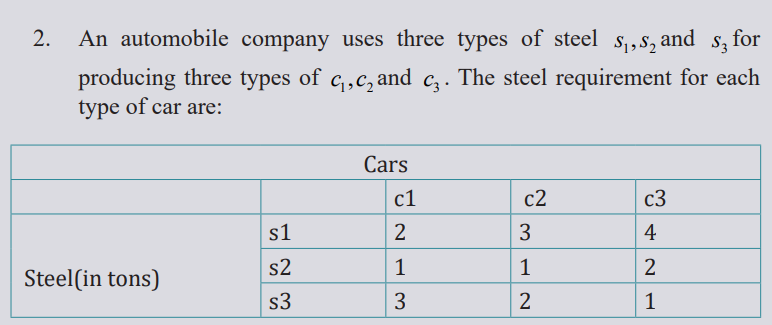
and 16 tons of steel of the three types respectively.
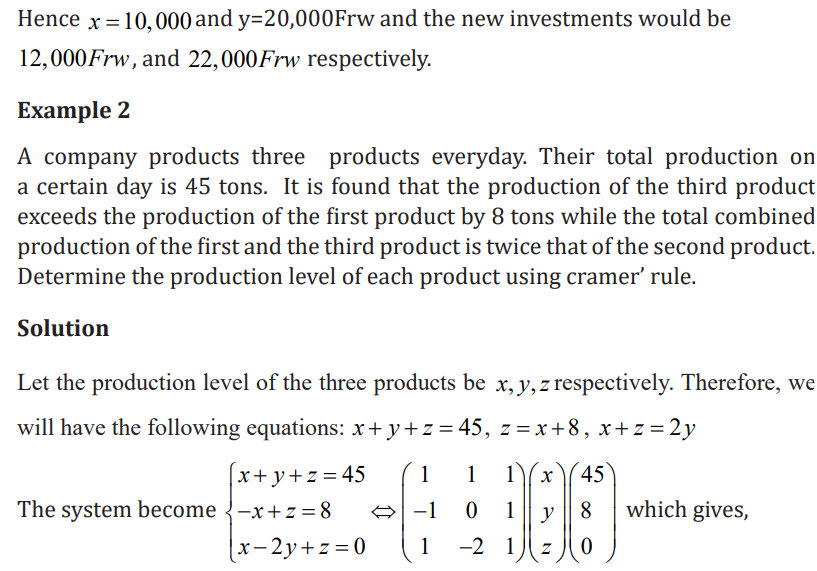
3. A company produces three products every day. Their total production
on a certain day is 45 tons. It is found that the production of the third
product exceeds the production of the first product by 8 tons while
the total combined production of the first and the third product is
twice that of the second product. Determine the production level ofeach product using Cramer’s rule.
4. An economy has two sectors, mining and electricity. For each unit
of output, mining requires 40% units of its own production and
20% units of electricity. Moreover, for each unit output, electricityrequires 20% units of mining and 0.6 units of its own production.
a) Determine the consumption matrix C for this economy
b) Find the inverse of I-C
c) Using the Leontief model, determine the production levels from
each sector that are necessary to satisfy a final demand of 20 unitsfrom mining and 10 units from electricity.
UNIT 2: LINEAR INEQUALITIES AND THEIR APPLICATION IN LINEAR PROGRAMMING PROBLEMS
Key unit competencies: Solve linear programming problems
Introductory activity
1. Formulate 3 examples of linear inequalities, then perform the following:
(a) Form a system of linear inequalities. (b) Represent them on Cartesian
plane. (c) Show their meet region. (d) Establish the linkage betweenthem.
2. The two production companies produce two different drinking products
that, after being prepared, are graded into three classes: high, medium,
and low-quality. The companies agreed to provide 1200 dozens of high-
quality, 800 dozens of medium-quality, and 2400 dozens of low-quality
drinks per day. Both companies had different operating procedures andtook weekends off. Their specifics are provided below.
Apply the linear inequality concepts to present the above information and
determine the hour per day each company be operated to fulfill the signedcontract.
2.1 Recall of linear inequalities
Learning activity 2.1
Note that:
– When the same real number is added or subtracted from each side ofinequality the direction of inequality is not changed.
The direction of the inequality is not changed if both sides are multiplied
or divided by the same positive real number and is reversed if both sidesare multiplied or divided by the same negative real number.
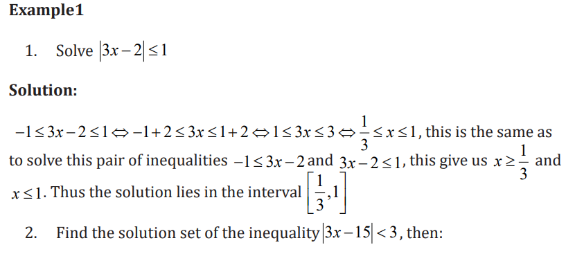

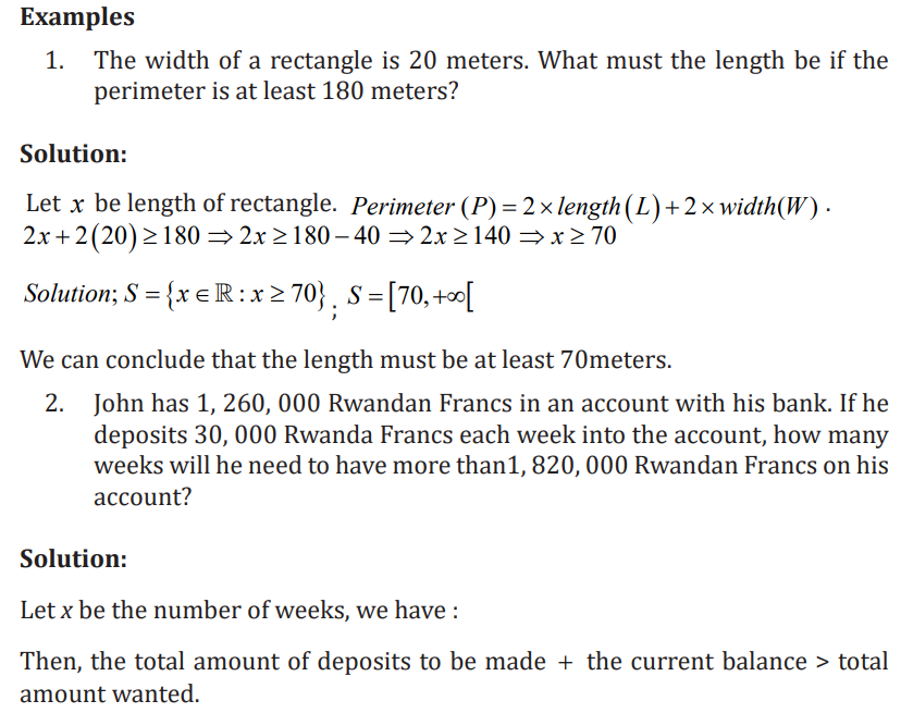
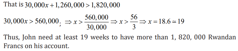
Problems involves linear inequalities
Inequalities can be used to model a number of real life situations. When
converting such word problems into inequalities, begin by identifying how the
quantities are relating to each other, and then pick the inequality symbol that is
appropriate for that situation. When solving these problems, the solution will
be a range of possibilities. Absolute value inequalities can be used to modelsituations where margin of error is a concern.
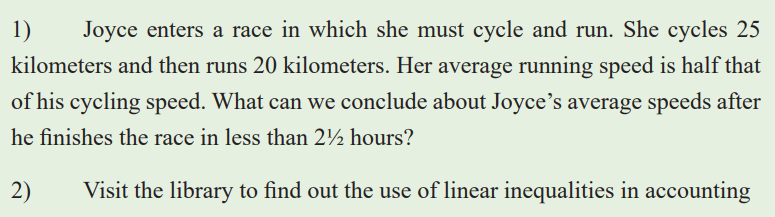
Application activity 2.1
2.2 Basic concepts of linear programming problem (LPP)
2.2.1 Definition and keys concepts
Learning activity 2.2.1
The following graph illustrate two lines and their equations, for each point
A, B, C, and D, replace its coordinate in the two inequalities to verify whichone satisfies the following system:
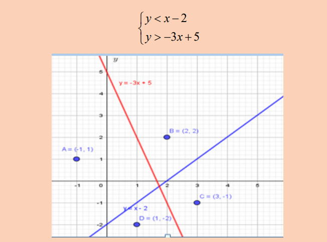
1. What are your observations on the graph as a future accountant?
2. Show the solution of these linear inequalities.
3. What is the common solution?
4. Where do we need this solution in Economics?
– A system of inequalities consits of a set of two or more inequalities with
the same variables. The inequalities define the conditions that are to beconsidered simultaneously.
– Each inequality in the set contains infinitely many ordered pair solutions
defined by a region in rectangular coordinate plane. When considering two
of these inequalities together, the intersection of these sets will define theset of simultaneous ordered pair solutions.
– A system of linear inequalities is similar to a system of linear equations,
except that it is made up of inequalities rather than equations. To modelscenarios with multiple constraints, systems of linear inequalities are used.
In finding solution, first, graphs the “equals” line, then shade in the correct
area. The following steps will be considered to find the solution of simultaneous
linear inequalities with two unknowns graphically, but for more than two isimpossible:
Linear inequalities with more than two unknowns are solved to find a range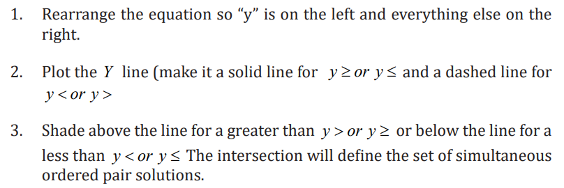
of values of three or more unknowns which make the inequalities true at the
same time. The solution is not represented graphically but we can apply one of
the following methods we expended in senior five Accounting, include Gaussian
elimination, comparison, substitution, or matrix inversion methods, and youare advised to review for recall on yourself.
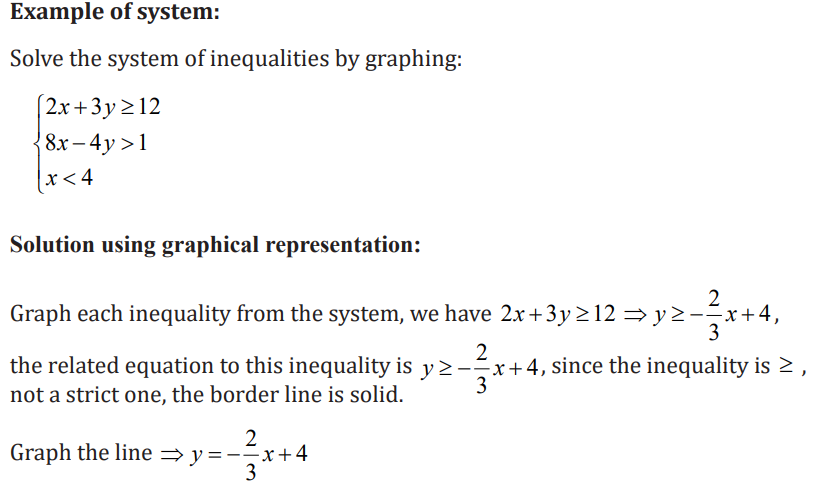

The solution of the whole system of inequalities is provided by the intersection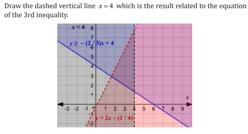
region of the solutions of all the three inequalities as it is shown in the figurebelow.
Linear programming is a subset of Operations Research (OR), an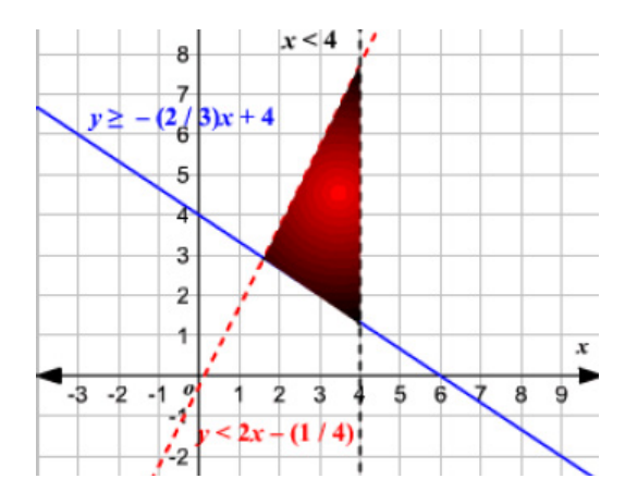
interdisciplinary branch of formal science that employs methods such as
mathematical modeling and algorithms to find optimal or near-optimal solutions
to complex problems. It has the goal of optimizing the solution (minimize costor maximize profit).
Therefore, Linear programming deals with the optimization (maximization or
minimization) of a function of variables known as objective function, subject
to a set of linear equalities and/or inequalities known as constraints. The
objective function may be profit, cost, production capacity or any other measureof effectiveness, which is to be obtained in the best possible or optimal manner.
Application activity 2.2.1
2.2.2 Mathematical models formulation and optimal solution
Learning activity 2.2.2
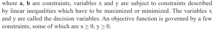
Refer to the application activity 2.2.1 where the transportation company
has signed a contract to transport at least 970 passengers and 370 tons of
luggage each trip and transport passengers in Rwanda with Bus A which is
capable of transporting 50 passengers and 40 tons of luggage, while Bus B
can only fit 70 passengers and 25 tons of luggage. If operating bus A costs
FRW1, 100,000 per trip and operating bus B costs FRW 1, 300,000 per trip.Then perform the following:
i. Without computation, which bus option will result in the lowestoverall cost per travel? Why?
ii. How can you reduce expenses?
A model in mathematics is simplified representation of an operation or a
process in which only the basic aspects or the most important features of a
typical problem under investigation are considered.
The objective of a model is to provide a means for analyzing the behaviour of
the system for the purpose of improving its performance. There are several
models in each area of business, or industrial activity. For instance, an account
model is a typical budget in which business accounts are referred to with the
intention of providing measurements such as rate of expenses, quantity sold,
etc.; A mathematical equation may be considered to be a mathematical modelin which a relationship between constants and variables is represented.
A model which has the possibility of measuring observations is called a
quantitative model; a product, a device or any tangible thing used forexperimentation may represent a physical model.
In this course Mathematical Model is used to model an object or situation from
the real world using mathematical ideas. It helps us understand the real world
and is used to improve many aspects of our lives. Mathematical models are an
essential part of the working world, from safety to planning and construction.
More broadly, a model is a representation of an object or idea that is used togain a better understanding of the real thing.
The procedures of translating any real world to mathematical problems are in
the table below.

Objective Function
The objective function is a mathematical equation that describes the production output
target that corresponds to the maximization of profits with respect to production. It
attempts to maximize profits or minimize losses based on a set of constraints andthe relationship between one or more decision variables. It is given by Z ax +by
Constraints
The objective function is subject to certain constraints, expressed by linear
inequalities. These constraints are actually the limitations on the primarydecision variables.
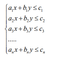
Each inequality constraint system determines a half-plane.
Feasible Solution
The feasibility region of the linear programming problem shows set of all
feasible solutions. A feasible solution of the linear programming problemsatisfies every constraint of the problem.
Corner points
Are the set of all points near feasible solution, and in these points we have to
choice the point which help us to maximize or minimize the objective functionas an optimal point.
Optimal Solution
It is also included in the feasible region; however, it represents the maximum
objective value of the function for the problem which requires maximization and
smallest objective value of the function that requires minimization. There are
many methods to solve linear programming problems. These methods include
a graphing method, Lagrange multipliers method, simplex method, northwest
corner method, and least cost method, etc. At this level, students will see only
how to solve problems using the graphical method only. Other methods will bestudied at the university level.
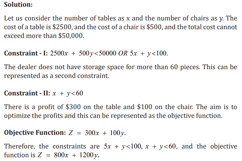
Example 1:
A furniture dealer has to buy chairs and tables and he has total available money
of $50,000 for investment. The cost of a table is $2500, and the cost of a chair is
$500. He has storage space for only 60 pieces, and he can make a profit of $300
on a table and $100 on a chair. Express this as an objective function and alsofind the constraints.
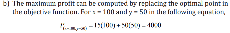
Example 2:
A furniture company produces office chairs and tables. The company projects
the demand of at least 100 chairs and 50 tables daily. The company can produce
no more than 120 chairs and 70 tables daily. The company must ship at most
150 units of chairs and tables daily to fulfill the shipping contract. Each soldtable results in the profit of 50 and each chair produces15 profit
a) How many units of chairs and tables should be made daily to maximizethe profit?
b) Compute the maximum profit the company can earn in a day?
Solution
a) Let x stands for the number of chairs sold daily, y stands for the numberof tables sold daily.
The objective function is given by P= 15x +50y ,

We graph the constraints inequalities on a Cartesian plane, and we obtain the following:
At point (100, 50) is there only one feasible solution which is also the optimal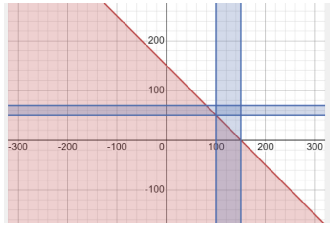
solution of the problem because all the three lines of the graph are intersecting
each other. Therefore, the point (100, 50) satisfies all the constraints of the
problem. Hence, a furniture company must produces 100 chairs and 50 tablesdaily to optimize the profits.
Application activity 2.2.2
A manufacturing company makes two kinds of instruments. The first
instrument requires 9 hours of fabrication time and one hour of labor
time for finishing. The second model requires 12 hours for fabricating
and 2 hours of labor time for finishing. The total time available for
fabricating and finishing is 180 hours and 30 hours respectively.
The company makes a profit of 800,000 Frw on the first instrument
and 1200, 000Frw on the second instrument. Express this linear
programming problem as an objective function and also find theconstraint involved.
2.3 Methods of solving linear programming problems (LPP)
2.3.1. Solving LPP using graphical methods
Learning activity 2.3.1
Learning activity 2.3.1
Consider the following problem
c) Which steps can you list to find solution? Graphically solve the givensystem of linear equation.
d) Do you think Profit can be shown from this graph?
To solve LPP we use graphical method under different steps. These are
summarized below:
Step 1. Identify the problem-the decision variables, the objective and therestrictions.
Step 2. Set up the mathematical formulation of the problem
Step 3. Plot a graph representing all the constraints of the problem and identify
the feasible region (solution space). The feasible region is the intersection of
all the regions bounded (represented) by the constraints of the problem and isrestricted to the first quadrant only.
Step 4. The feasible region obtained in step 3 may be bounded or unbounded.Compute the coordinates of all the corner points of the feasible region.
Step 5. Find out the value of the objective function at each corner (solution)point determined in step 4
Step 6. Select the corner point that optimizes (maximizes or minimizes) thevalue of the objective function. It gives the optimum feasible solution.
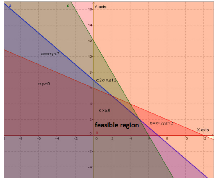
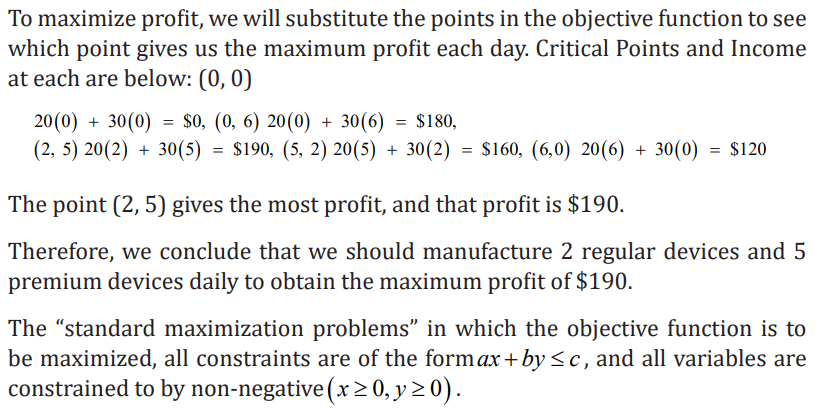
Example
A factory produces two types of devices including regular and premium. Each
device necessitates two operations, assembly and finishing, and each operation
has a maximum time limit of 12 hours. A standard device requires 1 hour of
assembly and 2 hours of finishing, whereas a premium device requires 2 hours
of assembly and 1 hour of finishing. Due to other constraints, the company can
only produce 7 devices per day. How many of each should be manufactured to
maximize profit if a profit of $20 is realized for each regular device and a profitof $30 for each premium device?

Application activity 2.3.1
Aline holds two part-time jobs, storekeeper, and Accountant. She never wants
to work more than a total of 12 hours a week. She has determined that for every
hour she works at storekeeper, she needs 2 hours of preparation time, and for
every hour she works at accountant, she needs one hour of preparation time,
and she cannot spend more than 16 hours for preparation. If Aline makes $40
an hour at Storekeeper, and $30 an hour at Accountant, how many hours shouldshe work per week at each job to maximize her income?
2.4 End unit assessment
1. An airline must sell at least 25 business class and 90 economy
class tickets to earn profit. It makes a profit of320 by selling each
business class ticket and a profit of 400 by selling an economy classticket. No more than 180 passengers can board the plane at a time.
i. How many of economy and business class tickets should be sold bythe airline to maximize the profit?
ii. How much maximum profit the airline can earn?
2. A bakery manufacturers two kinds of cookies, chocolate chip, and
caramel. The bakery forecasts the demand for at least 80 caramel
and 120 chocolate chip cookies daily. Due to the limited ingredients
and employees, the bakery can manufacture at most 120 caramel
cookies and 140 chocolate chip cookies daily. To be profitable the
bakery must sell at least 240 cookies daily. Each chocolate chip
cookie sold results in a profit of $0.75 and each caramel cookieproduces $0.88 profit.
i. How many chocolate chip and caramel cookies should be made dailyto maximize the profit?
ii. Compute the maximum revenue that can be generated in a day?
3. A farm is engaged in breeding pigs. The pigs are fed on various
products grown on the farm. In view of the need to ensure certain
nutrient constituents (call them A,B and C), it is necessary to buy
two additional products, say, X and Y. One unit of product X contains
36 units of A, 3 units of B and 20 units of C. One unit of product Y
contains 6 units of A, 12 units of B and 10 units of C. The minimum
requirement of A, B and C is 108 units, 36 units and 100 units
respectively. Product X costs 20FRW per unit and product Y costs
40 FRW per unit. Formulate the above as a linear Programming
problem to minimize the total cost, and solve the problem by using
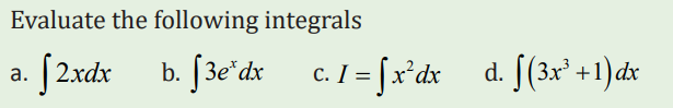
graphic method.UNIT 3: INTEGRALS
Key unit Competence: Use integration to solve mathematical and financial
related problems involving marginal cost, revenuesand profits, elasticity of demand, and supply
Introductory activity
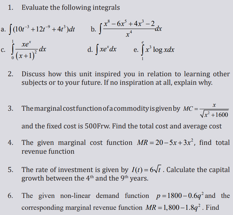
3.1 Indefinite integral
3.1.1 Definition and properties
Learning activity 3.1.1
Application activity 3.1.1
3.1.2 Properties of indefinite integral
Learning activity 3.1.2
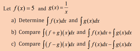
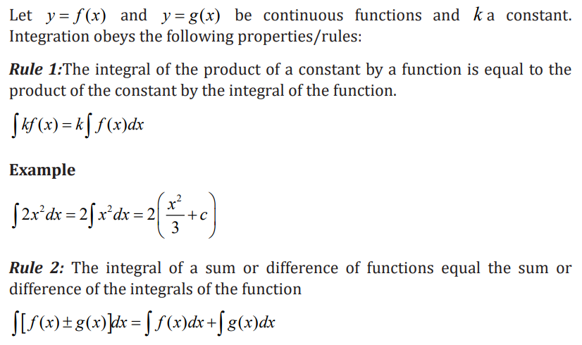
Note: Integration is a process which is the inverse of differentiation. In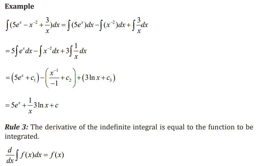
differentiation, we are given a function and we are required to find its derivative
or differential coeffient. In integration, we find a function whose differential
coeffient is given. The process of finding a function is called integration and itreverses the operation of differentiation.
Application activity 3.1.2

3.1.3 Primitive functions
Learning activity 3.1.3

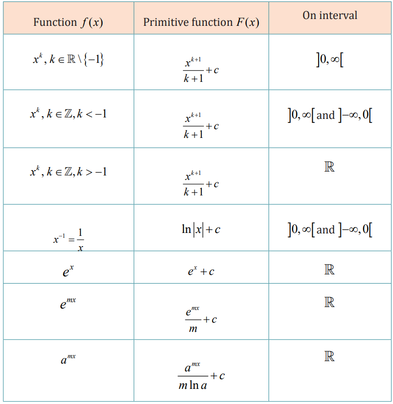

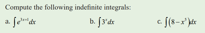
Application activity 3.1.3
3.2 Techniques of integration
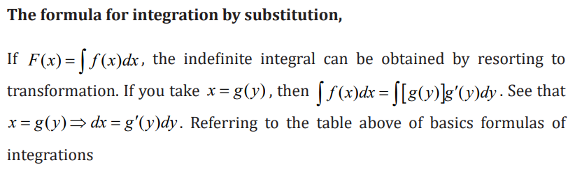
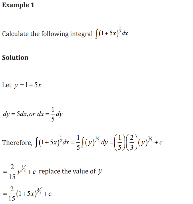
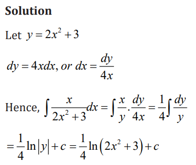
3.2.1 Integration by substitution or change of variable
Learning activity 3.2.1
Integration by substitution is based on rule of differentiating composite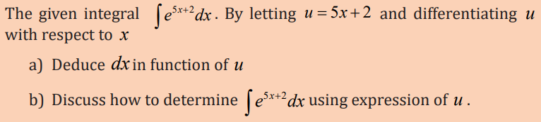
functions. As well as, any given integral is transformed into a simple form
of integral using this method of integration by substitution by substituting
other variables for the independent variable. When we make a substitution
for a function whose derivative is also present in the integrand, the method
of integration by substitution is extremely useful. As a result, the function
becomes simpler, and the basic integration formulas can be used to integratethe function.

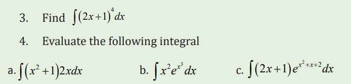
Application activity 3.2.1
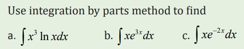
3.2.2 Integration by Parts
Learning activity 3.2.2
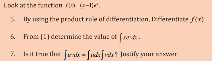
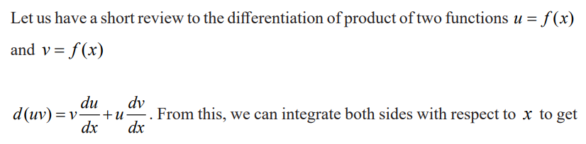
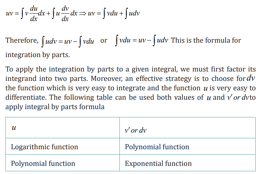

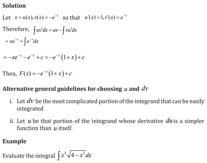

Application activity 3.2.2
3.2.3 Integration by Decomposition/ Simple fraction
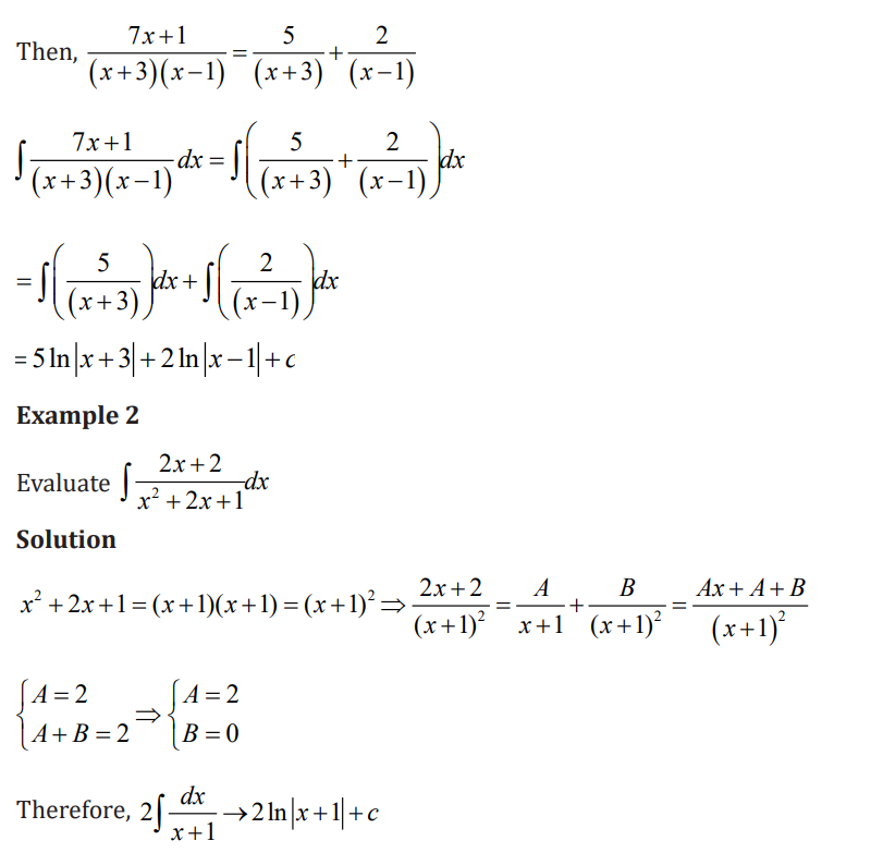
Learning activity 3.2.3
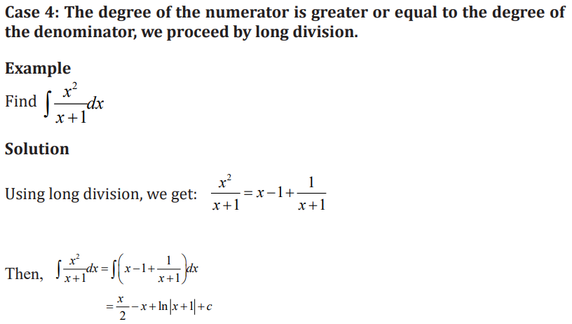
A rational expression is formed when a polynomial is divided by another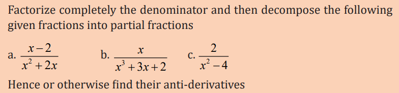
polynomial. In a proper rational expression, the degree of the numerator is
less than the degree of the denominator. In an improper rational expression,
the degree of the numerator is greater than or equal to the degree of the
denominator. The integration by decomposition known as integration of partial
fractions found by firstly decompose a proper fraction into a sum of simplerfractions.
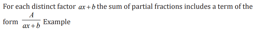
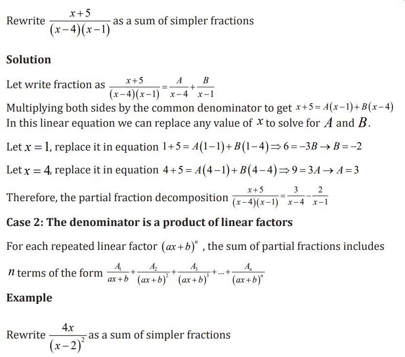
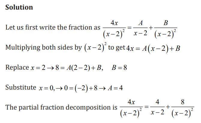
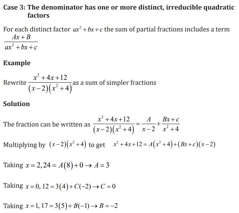
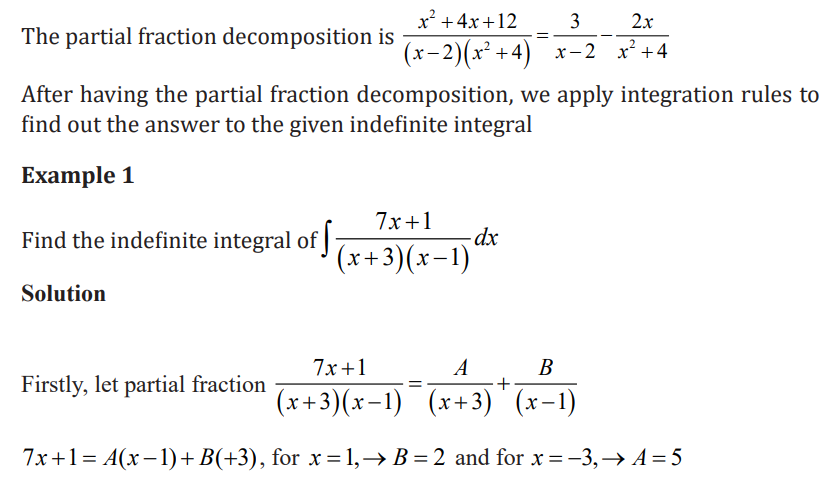
Partial fractions decomposition
CASE 1: The denominator is a product of distinct linear factors.
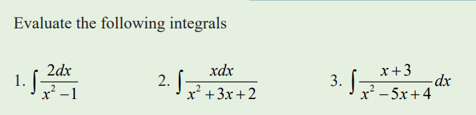
Application activity 3.2.3
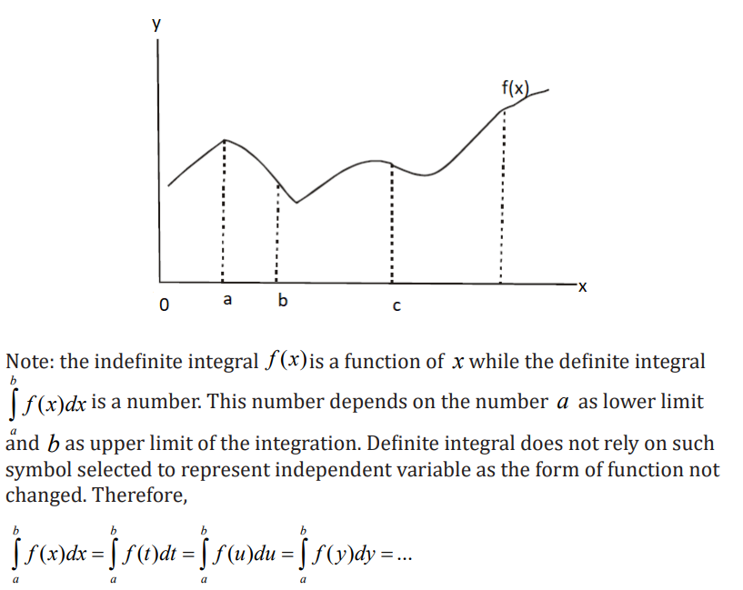
3.3. Definite integral
3.3.1 Definition and properties of definite integrals
Learning activity 3.3.1
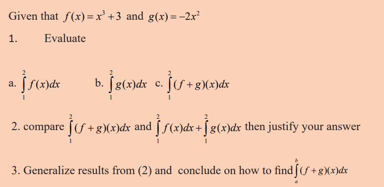

Application activity 3.3.1
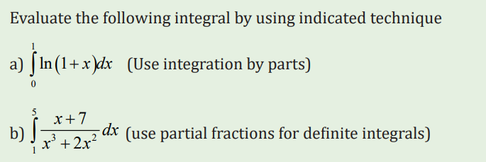
3.3.2 Techniques of integration of definite integral
Learning activity 3.3.2
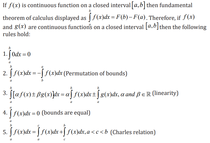
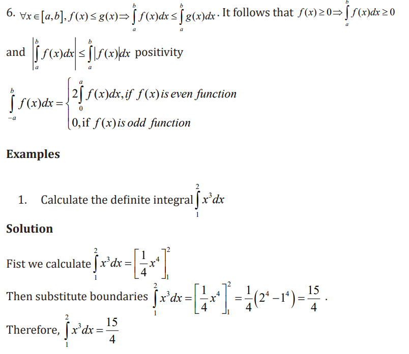
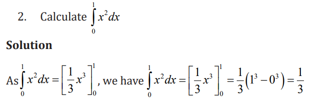
There is time that some functions cannot be integrated directly. In that case
we have to adopt other techniques in finding the integrals. The fundamental
theorem in calculus tells us that computing definite integral of f x
determining its anti-derivative, therefore the techniques used in determiningindefinite integrals are also used in computing definite integrals.
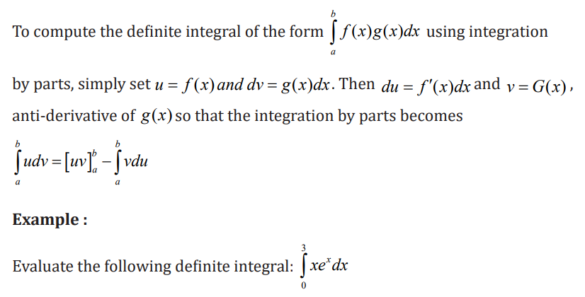
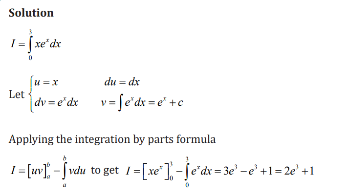
a) Integration by substitution
The method in which we change the variable to some other variable is called“Integration by substitution”.


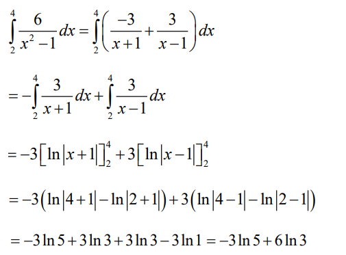
c) Decomposition or simple fractions
The partial fraction decomposition method is useful for integrating proper
rational functions. Divide our more complex rational fraction into smaller,
and more easily integrated rational functions. When splitting up the rational
function, the rules to follow are the same as from the indefinite integral. Here arethe steps for evaluating definite integrals using the method of partial fractions :
step 1: Factor the denominator of the integrand
step2: Split the rational function into a sum of partial fractions
step3: Set partial fractions decomposition equal to the original function
step 4: solve for numerators of each of the partial fractions
step 5: Take the definite integral of each of the partial fractions, and sumtogether

Application activity 3.3.2
3.4 Application of integration
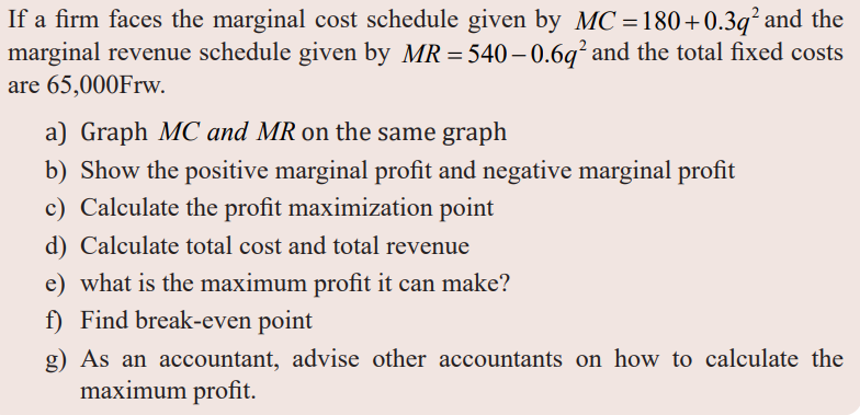
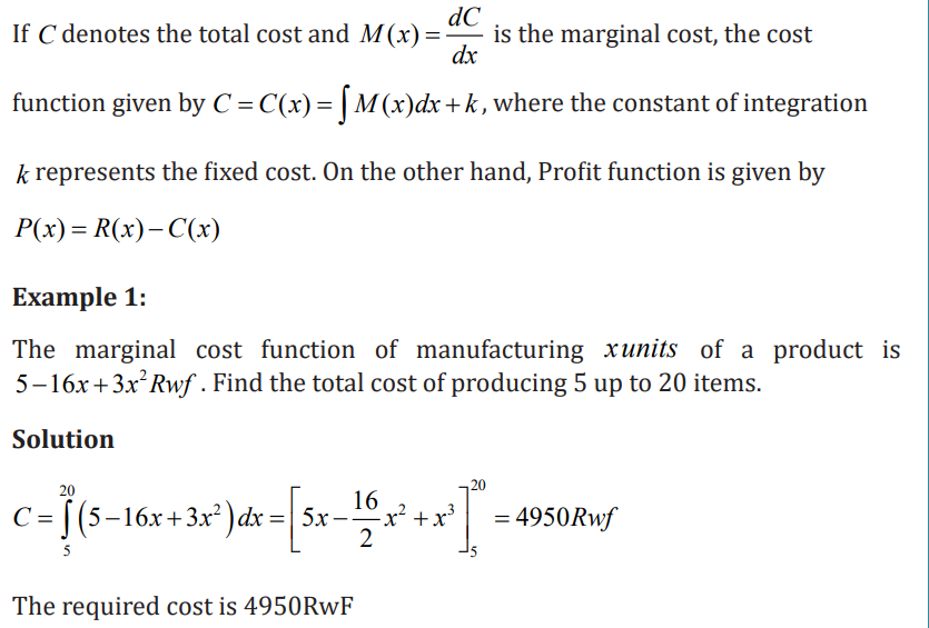
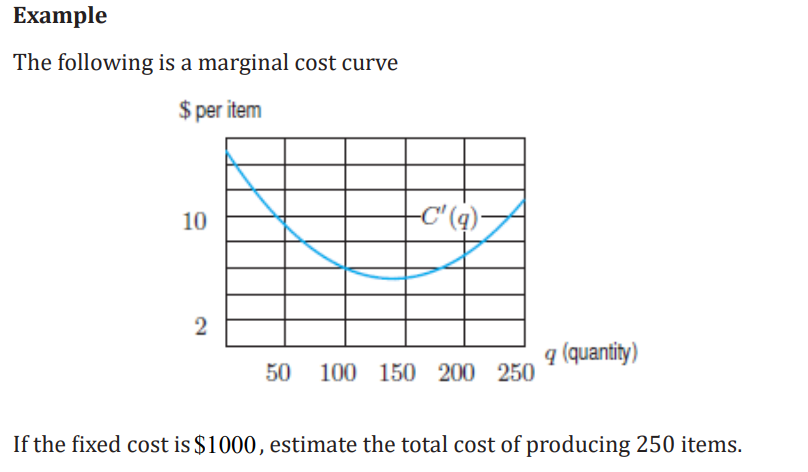
3.4.1 Calculation of marginal cost, revenues and profits
Learning activity 3.4.1
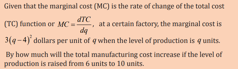
a) Cost function and profit function
If the variable under consideration varies continuously, integration allows us to
recover the total function from the marginal function. As a result, total functionssuch as cost, revenue, production, and saving can be derived from them.
The marginal function is obtained by differentiating the total function. Now,
when marginal function is given and initial values are given, the total functioncan be obtained using integration.


Solution
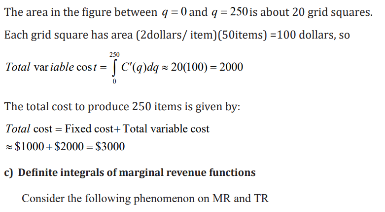
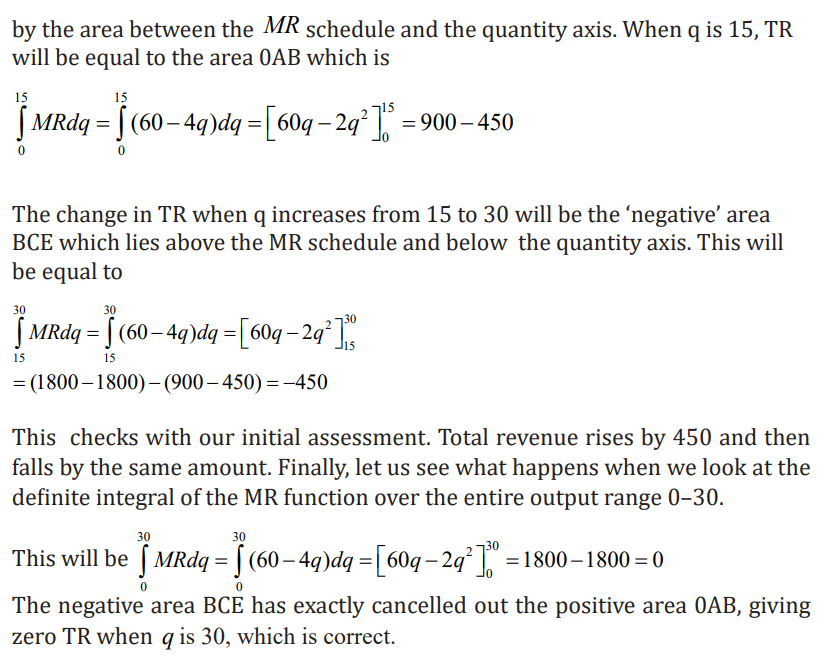
The total cost of production is fixed cost + Variable cost. The variable cost ofproducing 250 items is represented by the area under the marginal cost curve.
Application activity 3.4.1
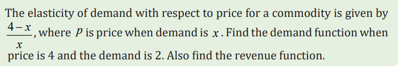
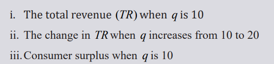
3.4.2 Elasticity of demand and supply
Learning activity 3.4.2
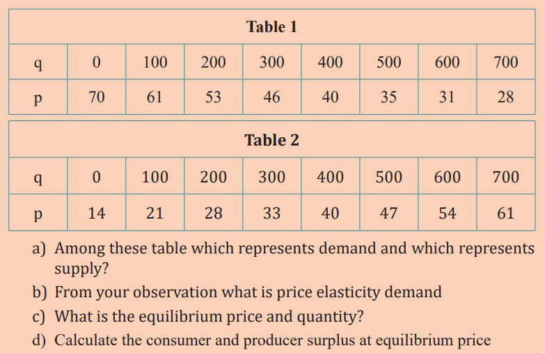
The table below shows information about the demand and supply
functions for a product. For both functions, q is the quantity and p is theprice, in dollars


Application activity 3.4.2
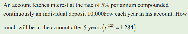
3.4.3 Present, Future Values of an Income Stream and Growth Rates
Learning activity 3.4.3
A company is considering purchasing a new machine for its production
floor. The machine costs $65,000. The company estimates that the
additional income from the machine will be a constant $7000 for the first
year, then will increase by $800 each year after that. In order to buy the
machine, the company needs to be convinced that it will pay for itself by
the end of 8 years with this additional income. Money can earn 1.7% peryear, compounded continuously. Should the company buy the machine?
to calculate the present and future value of a continuous income stream as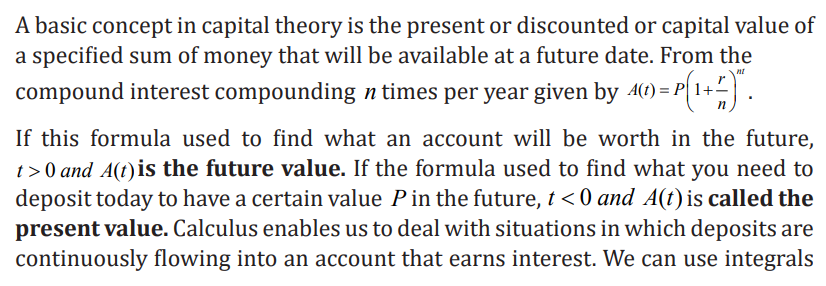
long as we can model the flow of income with a function. The idea here is that
each little bit of income in the future needs to be multiplied by the exponentialfunction to bring it back to the present, and then we’ll add them all up.

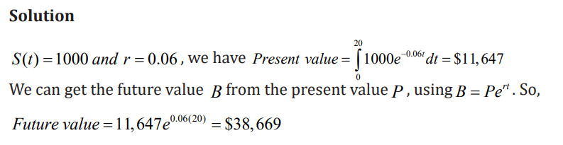
Example 2
Find the present and future values of a constant income stream of $1000 per
year over a period of 20 years, assuming an interest rate of 6% compoundedcontinuously
Further applications in production and consumption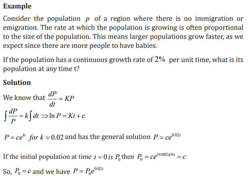
The supply function or supply curve shows the quantity of a product or service
that producers will supply over a period of time at any given price. Both theseprice-quantity relationships are usually considered as functions of quantity Q
Generally, the demand function P = D( Q) is decreasing, because consumers are
likely to buy more of a product at lower prices. Unlike the law of demand, the
supply function P = S(Q ) increasing, because producers are willing to deliver agreater quantity of a product at higher prices.
Application activity 3.4.3
3.5 End unit assessment
UNIT 4: INDEX NUMBERS AND APPLICATIONS
Key unit Competence: Apply index numbers in solving financial related
problems, interpreting a value index, and drawingappropriate decisions.
Introductory activity
An industrial worker was earning a salary of 100,000Frw in the year 2000.Today, he earns 1,200,000Frw.
i. Can his standard of living be said to have risen 12 times during thisperiod?
ii. Which statistical measure used to detect changes in a variable (risingor decreasing)
iii. By how much should his salary be raised so that he is as well off asbefore?
iv. Describe the methods can be used detect the rise of the price
4.1. Introduction to index numbers
4.1.1 Meaning, types and characteristics of index number
Learning activity 4.1.1
If a businessman wants to measure changes in the price level for a specific
group of consumers in his region of business.
a) Which statistical measure he can use to detect changes in a variable
or group of variables in his business
b) Help him how he can calculate consumer price index for industrial
workers, city workers and agricultural workers.1. Meaning of index number
An index number is a statistical measure used to detect changes in a variable
or group of variables. In addition, a single ratio (or percentage) that measures
the combined change of several variables between two different times, places,
or situations is referred to as an index number. Index numbers are expressedas percentages.
The relative change in price, quantity, or value in comparison to a base period.
An index number is used to track changes in raw material prices, employee andcustomer numbers, annual income and profits.
A simple index is one that is used to measure the relative change in only
one variable, such as wages per hour in manufacturing. A composite index
is a number that can be used to measure changes in the value of a group of
variables such as commodity prices, volume of production in different sectorsof an industry, production of various agricultural crops and cost of living.
The index number measures the average change in a group of related variables
over two different situations, such as commodity prices, volume of production
in various sectors of an industry, production of various agricultural crops, and
cost of living. Index numbers measure the changing value of a variable over
time in relation to its value at some fixed point in time, the base period, when itis given the value of 100
2. Characteristics of index numbers
Index numbers have the following important characteristics:
– Index numbers are of the type of average that measures the relative
changes in the level of a particular phenomenon over time. It is a special
type of average that can be used to compare two or more series made up ofdifferent types of items or expressed in different units.
– Index numbers are expressed as percentages to show the level of relativechange.
– Index numbers are used to calculate relative changes. They assess the
relative change in the value of a variable or a group of related variablesover time or between locations.
– Index numbers can also be used to quantify changes that are not directly
measurable. For example, the cost of living, price level, or business activity
in a country are not directly measurable, but relative changes in these
activities can be studied by measuring changes in the values of variables/factors that affect these activities.
3. Types of index numbers
a) Consumer price index
A consumer price index (CPI) tracks price changes in a basket of consumer
goods and services purchased by households. CPI measures changes in the price
level for a specific group of consumers in a given region. CPI can be calculated
for industrial workers, city workers and agricultural workers. Consumer priceindex is given by:
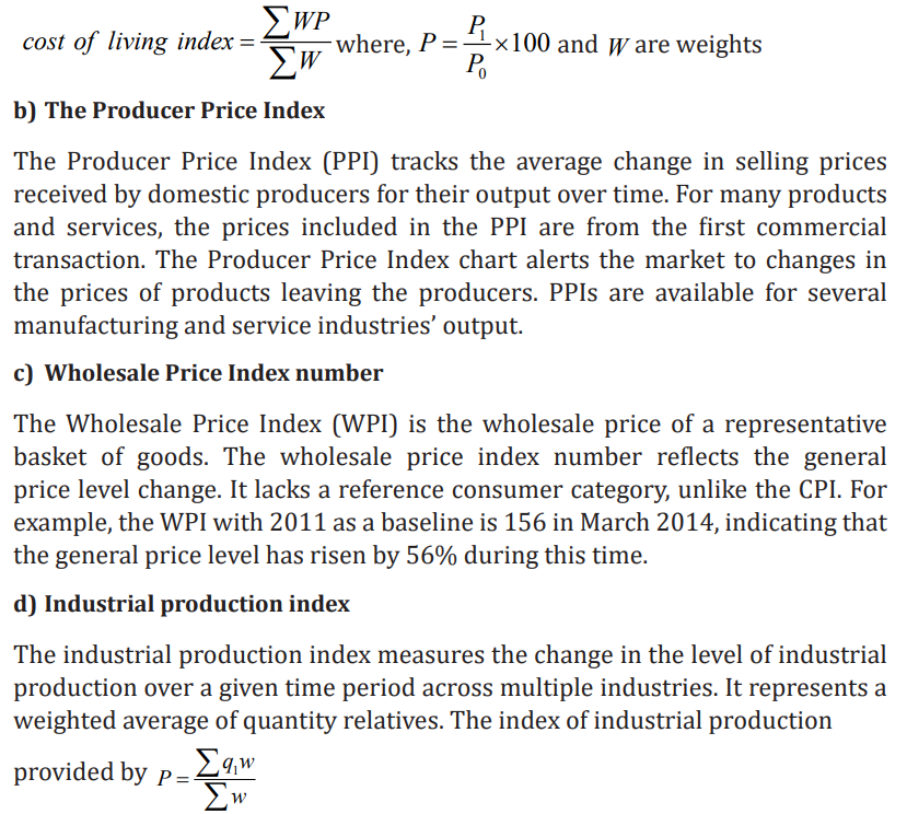
e) Uses of index numbers
The price indices such as CPI and PPI used to:
• Measure the cost of living;
• Measure of inflationary and deflationary tendencies in the economy,
• Means of adjusting income payments: nominal interest rates, wage
determination, taxes and other allowancesThe quantity/production Indices used to
• Used in national accounts to assess the performance of the economy
• Good indicator of the economic progress taking place in differentsectors, regions and countries to facilitate comparisons
Application activity 4.1.1
1. Discuss why index numbers are called as economic barometer2. Explain the characteristics of index number.
4.1.2. Construction of indices
Learning activity 4.1.2
For the given data of prices in certain country, answer the questions thatfollows:
a) How do you describe these prices over the given years?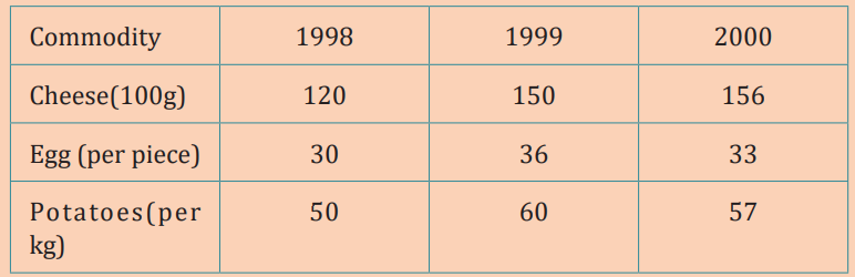
b) Describe the methods can be used to detect changes in these variable?
c) Find simple aggregative index for the year 1999 over the year 1998
d) Find the simple aggregative index for the year 2000 over the year1998
The construction of index numbers considers the definition of the purpose of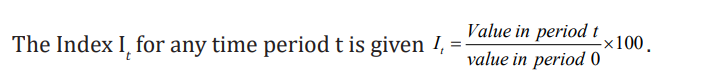
the index, selection of the base period, selection of commodities, obtaining price
quotations, choice of an average, selection of weights and then selection of a
suitable formula. Price index numbers are used to explain the various methods
of index number construction. Price index number construction methods canbe divided into three broad categories, as shown below:
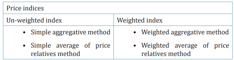
Un-weighted index
Weights are not assigned to the various items used in the calculation of the
un-weighted index number. The following are two un-weighted price indexnumbers:
i. Simple Aggregate Method
This method assumes that different items and their prices are quoted in the
same units. All of the items are given equal weight. The following is the formulafor a simple aggregative price index:
From the following data compute price index number for the year 2014 taking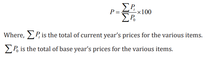
2013 as the base year using simple aggregative method:
This price index of 140 indicates that the aggregate of the prices of the given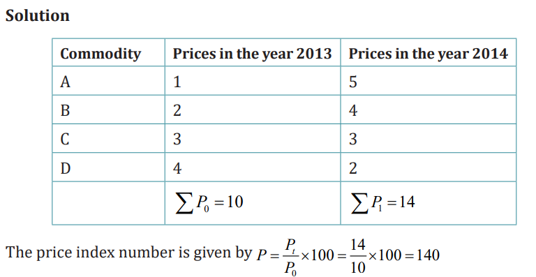
group of commodities increased by 40% between 2013 and 2014. This price
index number, calculated using a simple aggregative method, is only of limitedutility. The following are the reasons:
a) This method disregards the relative importance of the variouscommodities used in the calculation.
b) The various items must be expressed in the same unit. In practice, thevarious items may be expressed in different units.
c) The index number obtained by this method is untrustworthy because it
is influenced by the unit in which the prices of various commodities arequoted.
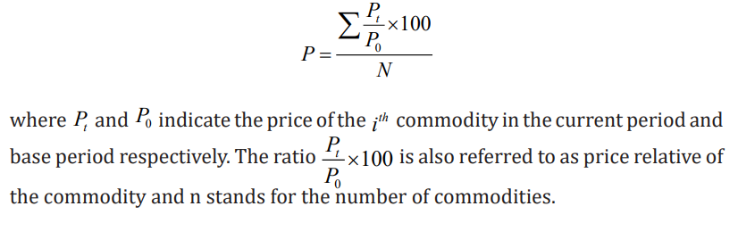
ii. Simple Average of Price Relatives Method
This method is superior to the previous one because it is unaffected by the
unit in which the prices of various commodities are quoted. Because the price
relatives are pure numbers, they are independent of the original units in which
they are quoted. The price index number is defined using price relatives asfollows:
Example1:
Using the data of example 1 the index number using price relative method canbe calculated as follows:
As a result, the price in 2014 is 112.5% higher than in 2013. The index number,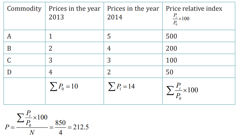
which is based on a simple average of price relatives, is unaffected by the units
in which the commodities’ prices are quoted. However, this method, like the
simple aggregative method, gives equal weight to all items, ignoring theirrelative importance in the group.
Weighted Index Number
All items or commodities are given rational weights in a weighted index number.
These weights indicate the relative importance of the items used in the index
calculation. In most cases, the quantity of usage is the most accurate indicatorof importance.
i. Weighted Aggregative Price Indices
Weights are assigned to each item in the basket in various ways in weighted
aggregative price indices, and the weighted aggregates are also used in various
ways to calculate an index. In most cases, the price index number is calculated
using the quantity of usage. The two most important methods for calculating
weighted price indices are Laspeyre’s price index and Paasche’s price index.
Laspeyre’s price index number is a weighted aggregative price index numberthat uses the quantity from the base year as the weights. It is provided by:
In the given example 2 (above), Paasche’s price index number can be calculated
as follows:
Weights in a weighted price relative index can be determined by the proportion
or percentage of total expenditure on them during the base or current period.
The base period weight is generally preferred over the current period weight.It is due to the inconvenience of calculating the weight every year.
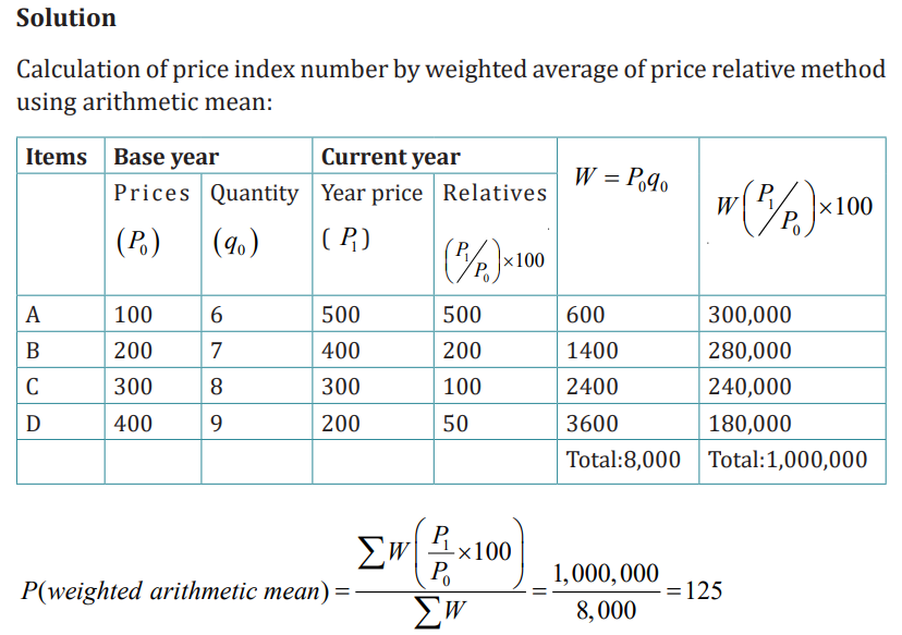
Example 3: From the following data compute an index number by usingweighted average of price relative method:
Application activity 4.1.2
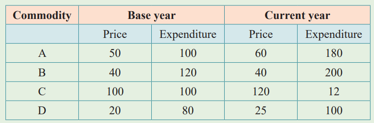
Compute Laspeyre’s and Paasche’s index numbers for 2000 from the followingdata
4.2 End unit assessment
1. Calculate cost of living index number using Family Budget method fromthe following data (Price in dollars).

i. Calculate the Laspeyre’s index
ii. Paasche’s index
3. Collect data from the local vegetable market over a week for, at
least 10 items. Try to construct the daily price index for the week.
What problems do you encounter in applying both methods for theconstruction of a price index?
UNIT 5: INTRODUCTION TO PROBABILITY
Key unit Competence: Use probability concepts to solve mathematical. Production,
financial, and economical related problems and drawappropriate decisions
Introductory activity
The following data were collected by counting the number of Warehouses in
use at MAGERWA over a 20 day period. 3 of the 20 days, only 1 Warehouse
was used, 5 of the 20 days, 2 Warehouses were used; 8 of the 20 days, 3
Warehouses were used; and 4 of the 20 days, 4 warehouses were used.
a) Construct a probability distribution for the data
b) Draw a graph for the probability distribution
c) Show that the probability distribution satisfies the required conditions for
a discrete probability distribution.d) On your own side defend why probability is important.
5.1. Key Concepts of probability
5.1.1. Definitions of probability terminologies
Learning activity 5.1.1
Consider the deck of 52 playing cards
1. Suppose that you are choosing one card
a) How many possibilities do you have for the cards to be chosen?
b) How many possibilities do you have for the kings to be chosen?
c) How many possibilities do you have for the aces of hearts to bechosen?
2. If “selecting a queen is an example of event, give other examples of
events.
Probability is random variable that can be happen or not, i.e. is the chance
that something will happen. Using the following examples, we can see how theconcept of probability can be illustrated in various contexts
Let us consider a game of playing cards. In a park of deck of 52 playing cards,
cards are divided into four suits of 13 cards each. If any player selects a card
by random (simple random sampling: chance of picking any card in the park is
always equal), then each card has the same chance or same probability of beingselected.
Second example, assume that a coin is tossed, it may show Head (H-face withlogo) or tail(T-face with another symbol), all these are mentioned below:
We cannot say beforehand whether it will show head up or tail up. The result
will depend on chance. The same, a card drawn from a well shuffled pack of 52
cards can be red or black. This also depends on chance. All these phenomena
are called probabilistic, means that can be occurred depending on the chance/uncertainty. The theory of probability is concerned with this type of phenomena.
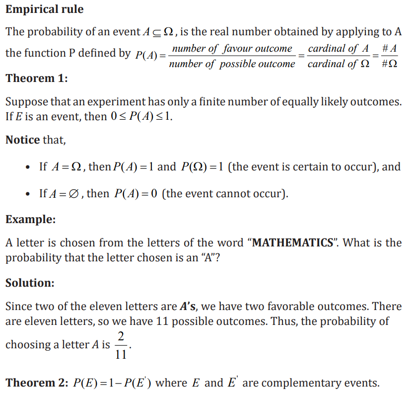
Probability is a concept which numerically measures the degree of uncertaintyand therefore certainty of occurrence of events.
In accounting, the sample of some documents and audited, then results
obtained in this sample will be generalized to the whole documents with
supporting recommendations to that particular accountant, institutions, andfurther decisions might be done basing on the findings obtained in the sample.
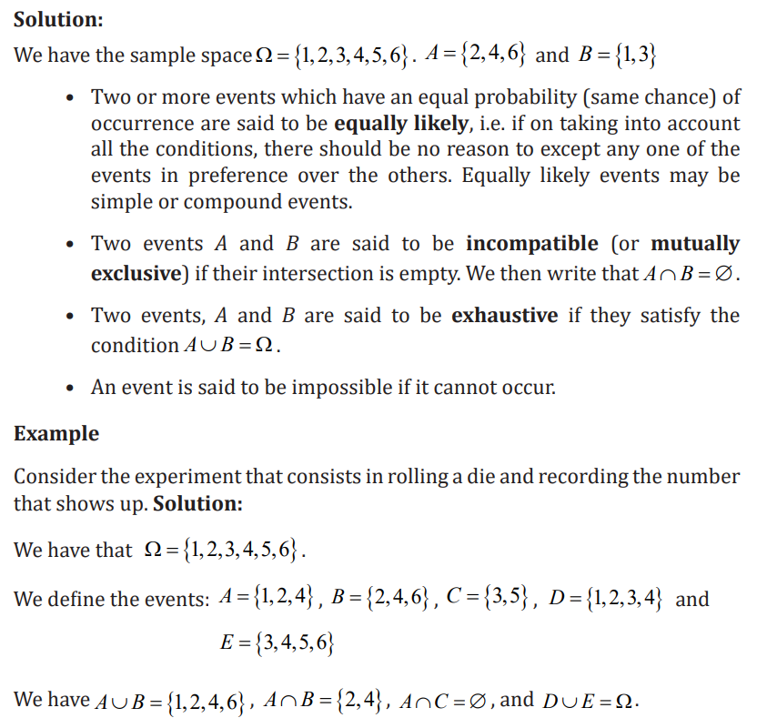
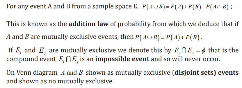
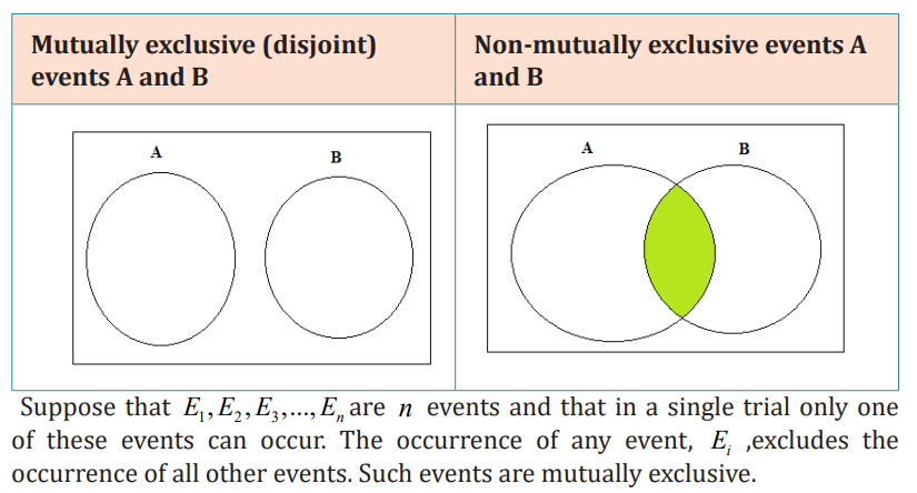
• Random experiments and Events
A random experiment is an experiment whose outcome cannot be predicted
or determined in advance. These are some example of experiments: Tossing
a coin, throwing a dice, selecting a card from a pack of paying cards, etc. In all
these cases there are a number of possible results (outcomes) which can occurbut there is an uncertainty as to which one of them will actually occur.
Each performance in a random experiment is called a trial. The result of a trial
in a random experiment is called an outcome, an elementary event, or a sample
point. The totality of all possible outcome (or sample points) of a random
experiment constitutes the sample space (the set of all possible outcomes of
a random experiment) which is denoted by Ω . Sample space may be discrete(single values), or continuous (intervals).
Discrete sample space:
• Firstly, the number of possible outcomes is finite.
• Secondly, the number of possible outcomes is countable infinite,
which means that there is an infinite number of possible outcomes,
but the outcomes can be put in a one-to-one correspondence with thepositive integers.
Continuous sample space
If the sample space contains one or more intervals, the sample space is thenuncountable infinite.
Example:
A die is rolled until a “6” is obtained and the time needed to get this first “6” is
recorded. In this case, we have to denote that
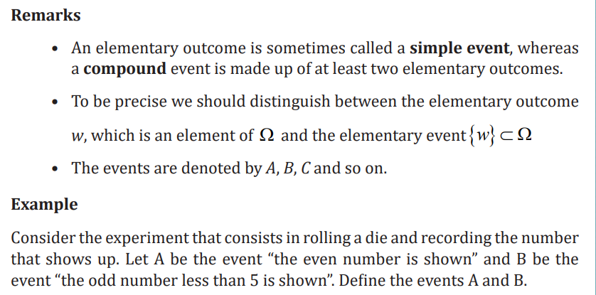
An event is a subset of the sample space. The null set φ is thus an event known
as the impossible event. The sample space Ω corresponds to the sure event.
In particular, every elementary outcome is an event, and so is the sample spaceitself.
Note: The determination of sample space for some events such as the one for
dice thrown simultaneously requires the use of complex reasoning but it can
be facilitated by different counting techniques. Morever,the number of possible
arrangements for a given set is calculated mathematically, and this process isknown as permutation.
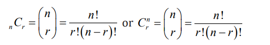
Permutation
Permutation is a term that refers to the variety of possible arrangements or
orders. The arrangement’s order is important when using permutations.
Permutations come in three varieties, one without repetition and two withrepetition. There is a way you can calculate permutations using a formula

Example 2
Consider a portfolio manager of a bank screened out 10 companies for a new
fund that will consist of 3 stocks. These 3 holdings will not be equal-weighted,
which means that ordering will take place. Help the manager to find out thenumber of ways to order the fund.

Combinations
In contrast to permutations, the combination is a method of choosing things
from a collection when the order of the choices is irrelevant. This means that a
combination is the choice of r things from a set of n things without replacementand where order does not matter.
Example
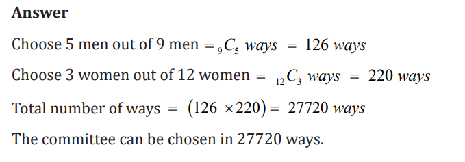
In a bank, the manager organizes election of bank committees consisting with
men and women. In how many ways a committee consisting of 5 men and 3women, can be chosen from 9 men and 12 women?
Application activity 5.1.1
1. A box contains 5 red, 3 blue and 2 green pens. If a pen is chosen at
random from the box, then which of the following is an impossible
event?
a) Choosing a red pen
b) Choosing a blue pen
c) Choosing a yellow pend) None of the above
2. Which of the following are mutually exclusive events when a day of
the week is chosen at random?
a) Choosing a Monday or choosing a Wednesday
b) Choosing a Saturday or choosing a Sunday
c) Choosing a weekday or choosing a weekend dayd) All of the above
3. Two dice are thrown simultaneously and the sum of points is noted,determine the sample space.
5.1.2. Empirical rules, axioms and theorems
Learning activity 5.1.2
Consider the letters of the word “PROBABILITY”.
a) How many letters are in this word?
b) How many vowels are in this word?
c) What is the ratio of numbers of vowels to the total number of letters?
d) How many consonants are in this word?
e) What is the ratio of numbers of consonants to the total number of
letters?f) Let A be the set of all vowels and B the set of all consonants. Find
i. A ∩B
ii. A ∪B
iii. A'
iv. B'
Application activity 5.1.2
1. A letter is chosen from the letters of the word “MATHEMATICS”.What is the probability that the letter chosen is M? and T?
2. An integer is chosen at random from the set
S = {all positive integers less than 20} . Let A be the event of choosinga multiple of 3 and let B be the event of choosing an odd number. Find
a) P ( A∪ B)
b) P (A ∩B )
c) P (A − B)
5.1.3 Additional law of probability, Mutual exclusive, and exhaustive
Learning activity 5.1.3
Consider a machine which manufactures car components. Suppose each
component falls into one of four categories: top quality, standard,substandard, reject
After many samples have been taken and tested, it is found that under certain
specific conditions the probability that a component falls into a category is
as shown in the following table. The probability of a car component fallinginto one of four categories.
The four categories cover all possibilities and so the probabilities must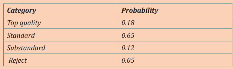
sum to 1. If 100 samples are taken, then on average 18 will be topquality, 65 of standard quality, 12 substandard and 5 will be rejected.
Using the data in table determine the probability that a component selectedat random is either standard or top quality.

Solution:
Since only one person wins, the events are mutually exclusive.
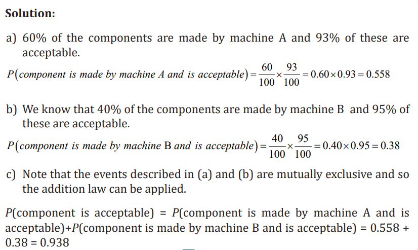
3. Machines A and B make components. Machine A makes 60% of the
Components. The probability that a component is acceptable is 0.93 when
made by machine A and 0.95 when made by machine B. A component ispicked at random. Calculate the probability that it is:
a) Made by machine A and is acceptable.
b) Made by machine B and is acceptable.c) Acceptable.
Application activity 5.1.3
1. A fair die is rolled, what is the probability of getting an even numberor prime number?
2. Events A and B are such that they are both mutually exclusive andexhaustive. Find the relation between these two events.
3. In a class of a certain school, there are 12 girls and 20 boys. If a
teacher want to choose one student to answer the asked question
a) What is the probability that the chosen student is a girl?
b) What is the probability that the chosen student is a boy?
c) If teacher doesn’t care on the gender, what is the probability ofchoosing any student?
4. On New Year’s Eve, the probability of a person driving while
intoxicated is 0.32, the probability of a person having a driving
accident is 0.09, and the probability of a person having a drivingaccident while intoxicated is 0.06.
What is the probability of a person driving while intoxicated or having adriving accident?
5.1.4 Independence, Dependence and conditional probability
Learning activity 5.1.4
Suppose that you have a deck of cards; then draw a card from that deck,not replacing it, and then draw a second card.
a) What is the sample space for each event?
b) Suppose you select successively two cards, what is the probability ofselecting two red cards?
c) Explain if there is any relationship (Independence or dependence)
between those two events considering the sample space. Does theselection of the first card affect the selection of the second card?


Contingency table
Contingency table (or Two-Way table) provides a different way of calculating
probabilities. It helps in determining conditional probabilities quite easily. The
table displays sample values in relation to two different variables that may bedependent or contingent on one another.
Below, the contingency table shows the favorite leisure activities for 50 adults,
20 men and 30 women. Because entries in the table are frequency counts, thetable is a frequency table.
Entries in the total row and total column are called marginal frequencies or
the marginal distribution. Entries in the body of the table are called jointfrequencies.
Example
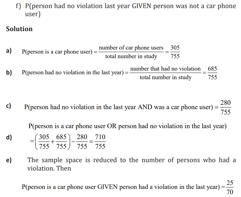
Suppose a study of speeding violations and drivers who use car phonesproduced the following fictional data:
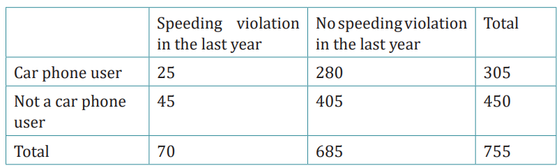
Calculate the following probabilities using the table:
a) P(person is a car phone user)
b) P(person had no violation in the last year)
c) P(person had no violation in the last year AND was a car phone user)
d) P(person is a car phone user OR person had no violation in the last year)
e) P(person is a car phone user GIVEN person had a violation in the lastyear)
Application activity 5.1.4
1. A dresser drawer contains one pair of socks with each of the
following colors: blue, brown, red, white and black. Each pair is
folded together in a matching set. You reach into the sock drawer
and choose a pair of socks without looking. You replace this pair
and then choose another pair of socks. What is the probability thatyou will choose the red pair of socks both times?
2. A coin is tossed and a single 6-sided die is rolled. Find the probabilityof landing on the head side of the coin and rolling a 3 on the die.
4. The world-wide Insurance Company found that 53% of the residents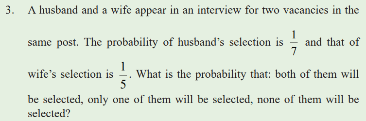
of a city had home owner’s Insurance with its company of the
clients, 27% also had automobile Insurance with the company. If a
resident is selected at random, find the probability that the resident
has both home owner’s and automobile Insurance with the worldwide Insurance Company.
5. Calculate the probability of a 6 being rolled by a die if it is alreadyknown that the result is even.
6. A jar contains black and white marbles. Two marbles are chosen without
replacement. The probability of selecting a black marble and then a
white marble is 0.34, and the probability of selecting a black marble on
the first draw is 0.47. What is the probability of selecting a white marbleon the second draw, given that the first marble drawn was black?
5.1.5. Tree diagram, Bayes theorem and its applications
Learning activity 5.1.5
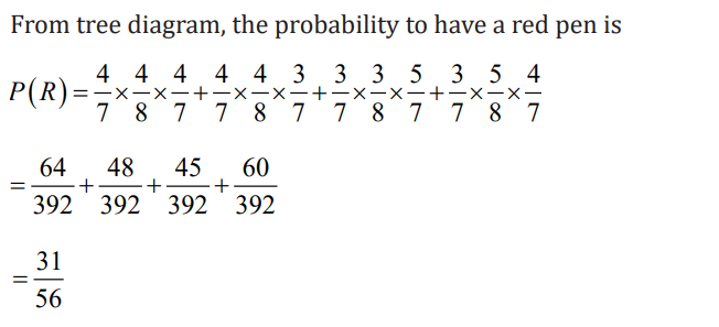
1. A box contains 4 blue pens and 6 black pens. One pen is drawn at
random, its color is noted and the pen is replaced in the box. A pen isagain drawn from the box and its color is noted.
a) For the 1st trial, what is the probability of choosing a blue pen andprobability of choosing a black pen?
b) For the 2nd trial, what is the probability of choosing a blue pen and
probability of choosing a black pen? Remember that after the 1st trialthe pen is replaced in the box.
2. In the following figure complete the missing colours and probabilities
a) Tree diagram
A tree diagram is a tool in the fields of probability, and statistics that helps
calculate the number of possible outcomes of an event or problem, and to
cite those potential outcomes in an organized way. It can be used to show the
probabilities of certain outcomes occurring when two or more trials take
place in succession. The outcome is written at the end of the branch and the
fraction on the branch gives the probability of the outcome occurring. For each
trial the number of branches is equal to the number of possible outcomes ofthat trial. In the diagram there are two possible outcomes, A and B, of each trial.
Successive trials are events which are performed one after the other; all ofwhich are mutually exclusive.
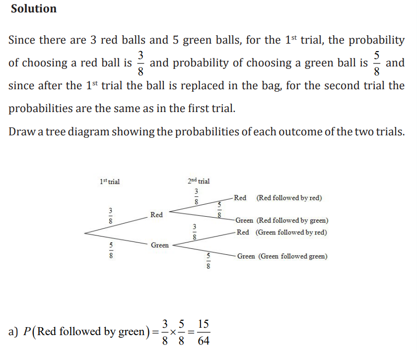
Examples:
1. A bag contains 8 balls of which 3 are red and 5 are green. One ball is
drawn at random, its color is noted and the ball replaced in the bag. A ball
is again drawn from the bag and its color is noted. Find the probabilitythe ball drawn will be
a) Red followed by green,
b) Red and green in any order,c) Of the same color

Application activity 5.1.5
1. Calculate the probability of three coins landing on: Three heads.
2. A class consists of six girls and 10 boys. If a committee of three
is chosen at random, find the probability of: a) Three boys being
chosen, b) exactly two boys and a girl being chosen. Exactly twogirls and a boy being chosen, d) three girls being chosen.
3. A bag contains 7 discs, 2 of which are red and 5 are green. Two discs
are removed at random and their colours noted. The first disk is not
replaced before the second is selected. Find the probability that thediscs will be
a) both red, b) of different colours, c) the same colours.
4. Three discs are chosen at random, and without replacement, from a
bag containing 3 red, 8 blue and 7 white discs. Find the probability
that the discs chosen will bea) all red b) all blue c) one of each colour.
5. 20% of a company’s employees are engineers and 20% are
economists. 75% of the engineers and 50% of the economists hold
a managerial position, while only 20% of non-engineers and non-
economists have a similar position. What is the probability that
an employee selected at random will be both an engineer and amanager?
6. The probability of having an accident in a factory that triggers an
alarm is 0.1. The probability of its sounding after the event of an
incident is 0.97 and the probability of it sounding after no incident
has occurred is 0.02. In an event where the alarm has been triggered,what is the probability that there has been no accident?
5.2. Probability distributions
5.2.1 Discrete probability distribution
Learning activity 5.2.1
Learning activity 5.2.1
In City of Kigali, data were collected on the number of people who had
applied to buy shares in the Rwanda Stock Exchange. People bought
different shares although some withdrew their requests. The table belowshows the collected data.
Develop the probability distribution of the random variable defined as the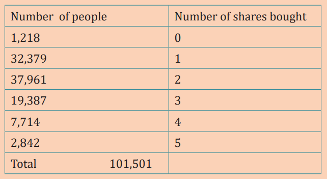
number of shares bought per person.
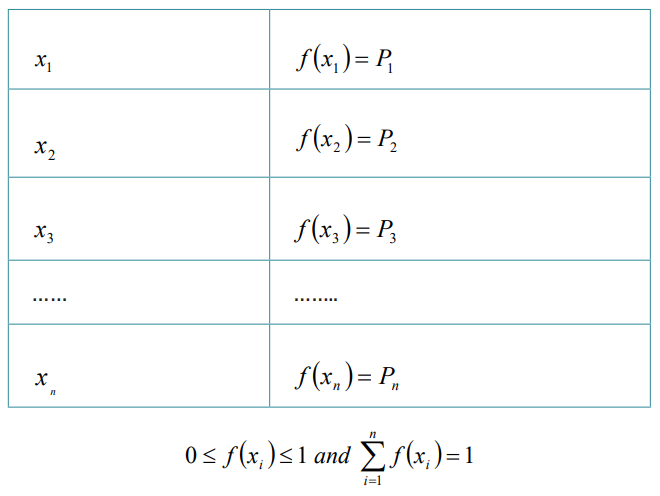
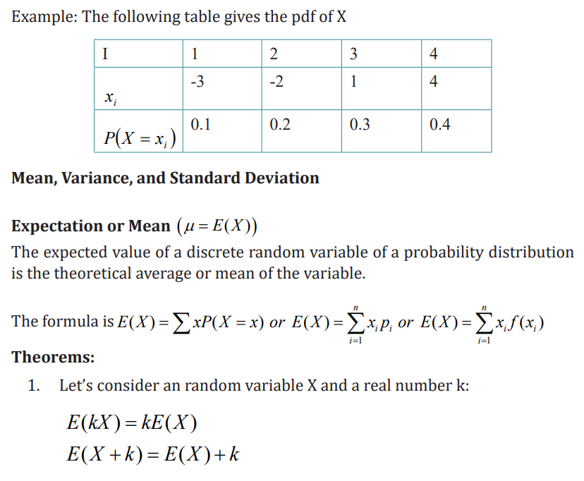
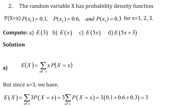
Probability Distribution: The values a random variable can assume and the
corresponding probabilities of each. Probability distributions are related tofrequency distributions.
For a discrete random variable x, the probability distribution is defined
by a probability function, denoted by f(x). The probability function gives theprobability for each value of the random variable. Then X is a discrete random
A discrete Variable is a variable that can take on a finite or countable number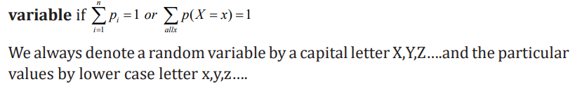
of distinct values. It is a variable that is characterized by gaps in the values itcan take.
Examples
– number of heads observed in an experiment that flips a coin 10 times,
– number of times a student visits the library;– number of children in class
A discrete probability distribution consists of the values a random variable
can assume and the corresponding probabilities of the values. The probabilitiesare determined theoretically or by observation.
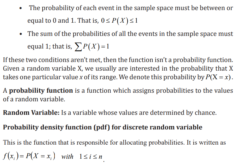
Two Requirements for a Probability Distribution are


Application activity 5.2.1
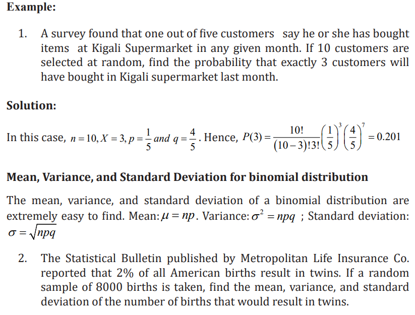
5.2.2 Binomial Distribution
Learning activity 5.2.2
With your potential explanations and examples to fit the following fourconditions:
• A fixed number of trials
• Each trial is independent of the others
• There are only two outcomes
• The probability of each outcome remains constant from trial totrial.
Binomial distribution is calculated by multiplying the probability of success raised
to the power of the number of successes and the probability of failure raised to thepower of the difference between the number of successes and the number of trials.
Let consider an experiment with independent trials and only two possible

Application activity 5.2.2
1. A multiple-choice test with 20 questions has five possible answers
for each question. A completely unprepared student picks the
answers for each question at random and independently. SupposeX is the number of questions that the student answers correctly.
Calculate the probability that:
a) The student gets every answer wrong.
b) The student gets every answer right.c) The student gets 8 right answers.
2. An examination consisting of 10 multiple choice questions is to
be done by a candidate who has not revised for the exam. Eachquestion has five possible answers out of which only one is correct.
The candidate simply decides to guess the answers.
i. What is the probability that the candidate gets no answer correct?
ii. What is the probability that the student gets two correct answers?
3. Suppose you took three coins and tossed them in the air.
a) show all the possible outcomes when the coin is tossed
b) What is the probability that all three will come up heads?
c) What is the probability of 2 heads?
d) Show the probability distribution on a graph (use the number ofheads)
5.2.3 Bernoulli distribution
Learning activity 5.2.3
On your own, can you suggest the Bernoulli examples, using the binomialexperiment shown above? What are your differences and Similarities?
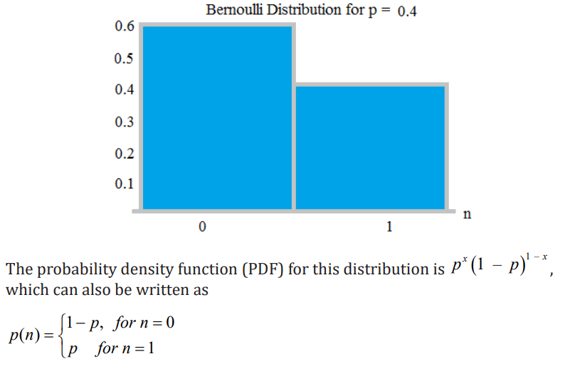
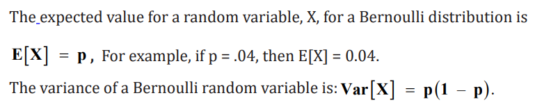
A Bernoulli distribution is a discrete probability distribution for a Bernoulli
trial. A Bernoulli trial is one of the simplest experiments you can conduct. It’s
an experiment where you can have one of two possible outcomes. For example,“Yes” and “No” or “Heads” and “Tails.
A random experiment that has only two outcomes (usually called a “Success”
or a “Failure”). For example, the probability of getting a heads (a “success”)
while flipping a coin is 0.5. The probability of “failure” is 1 – P (1 minus the
probability of success, which also equals 0.5 for a coin toss). It is a special case of
the binomial distribution for n 1 = . In other words, it is a binomial distributionwith a single trial (e.g. a single coin toss).
For example
In the following Bernoulli distribution, the probability of success (1) is 0.4, andthe probability of failure (0) is 0.6
Application activity 5.2.3
Provide any examples describing discrete not continuous data resulting
from an experiment known as Bernoulli process/trials in your areas ofinterest as accounting professional.
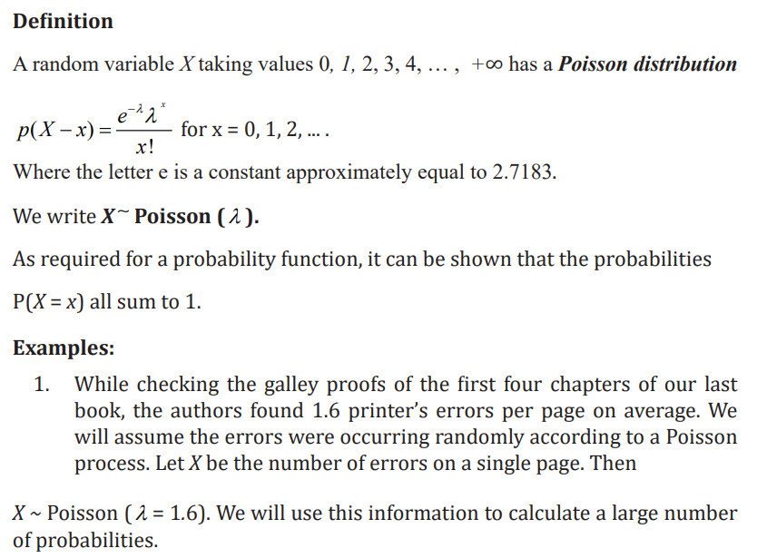
5.2.4 Poison distribution
Learning activity 5.2.4
Describe the characteristics of the following examples:
a) The number of cars arriving at a service station in 1 hour;
b) The number of accidents in 1 day on a particular stretch of high way.
c) The number of visitors arriving at a party in 1 hour,
d) The number of repairs needed in 10 km of road,
e) The number of words typed in 10 minutes.f) Why these skills and knowledge are needed in Accounting professional.
Considering the binomial distribution, the values of p and q and n are given.
If there are cases where p is very small and n is very large, then calculation
involved will be long. Such cases will arise in connection with rare events, forexample.
• Persons killed in road accidents;
• The number of defective articles produced by a quality machine;
• The number of mistakes committed by a good typist, per page;
• The number of persons dying due to rare disease or snake bite;
• The number of accidental deaths by falling from trees or roofs etc.
In all these cases we know the number of times an event happened but not
how many times it does not occur. Events of these types are further illustratedbelow:
1. It is possible to count the number of people who died accidently by
falling from trees or roofs, but we do not know how many people did notdie by these accidents.
2. It is possible to know or to count the number of earth quakes that
occurred in an area during a particular period of time, but it is, more or
less, impossible to tell as to how many times the earth quakes did notoccur.
3. It is possible to count the number of goals scored in a foot-ball match butcannot know the number of goals that could have been but not scored.
4. It is possible to count the lightning flash by a thunderstorm but it is
impossible to count as to how many times, the lightning did not flash etc.
Thus n, the total of trials in regard to a given event is not known, the binomialdistribution is inapplicable,
Poisson distribution is made use of in such cases where p is very small. We
mean that the chance of occurrence of that event is very small. The occurrence
of such events is not haphazard. Their behavior can also be explained by
mathematical law. Poisson distribution may be obtained as a limiting case ofbinomial distribution.

Application activity 5.2.4
1. A lecturer of statistics has observed that the number of typing
errors in new edition of text books varies considerably from book to
book. After some analysis we conclude that the number of errors is
a Poisson distribution with a mean 1.5 per 100 pages. The lecturer
randomly selects 100 pages of a new book. What is the probabilitythat there are no typing errors?
2. If there are 200 typographical errors randomly distributed in a 500-
page manuscript, find the probability that a given page containsexactly 3 errors.
3. The mean number of bacteria per millimeter of a liquid is known
to be 4. Assuming that the number of bacteria follows a Poisson
distribution, find the probability that 1 ml of liquid there will be: Nobacteria, 4 bacteria, less than 3 bacteria
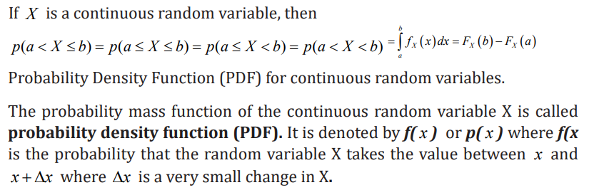
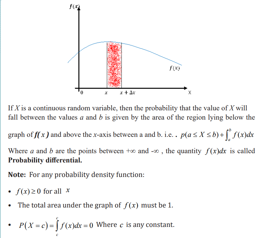
5.2.5 Continuous Probability Distributions
Learning activity 5.2.5
A continuous random variable is a theoretical representation of a continuous
variable such as height, mass or time.
Examples
• the amount of time to complete a task.
• Heights of trees in a school garden
• Daily temperature• Interest earned daily on bank loans per person
Application activity 5.2.5
5.2.6 Normal distribution
Learning activity 5.2.6
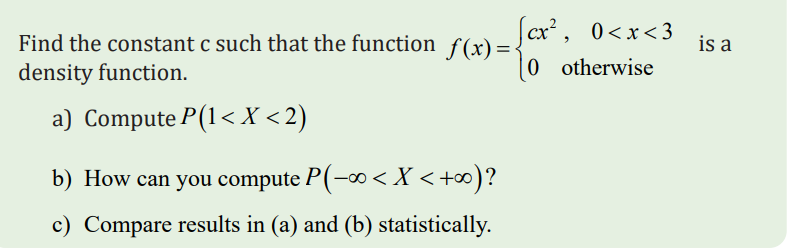
Explain clearly the results shown above, how these findings are linked to
probability distributions? Can you compare descriptive statistics and thisprobability distribution as an accountant? How?
Definitions
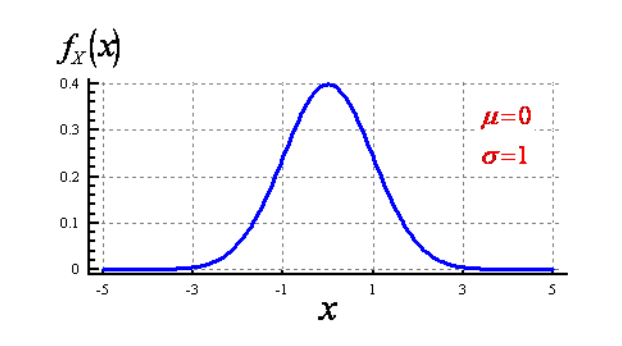
A normal distribution is a continuous, symmetric, bell-shaped distribution ofa variable.
Standard Error or the Mean: The standard deviation of the sampling
distribution of the sample means. It is equal to the standard deviation of thepopulation divided by the square root of the sample size.
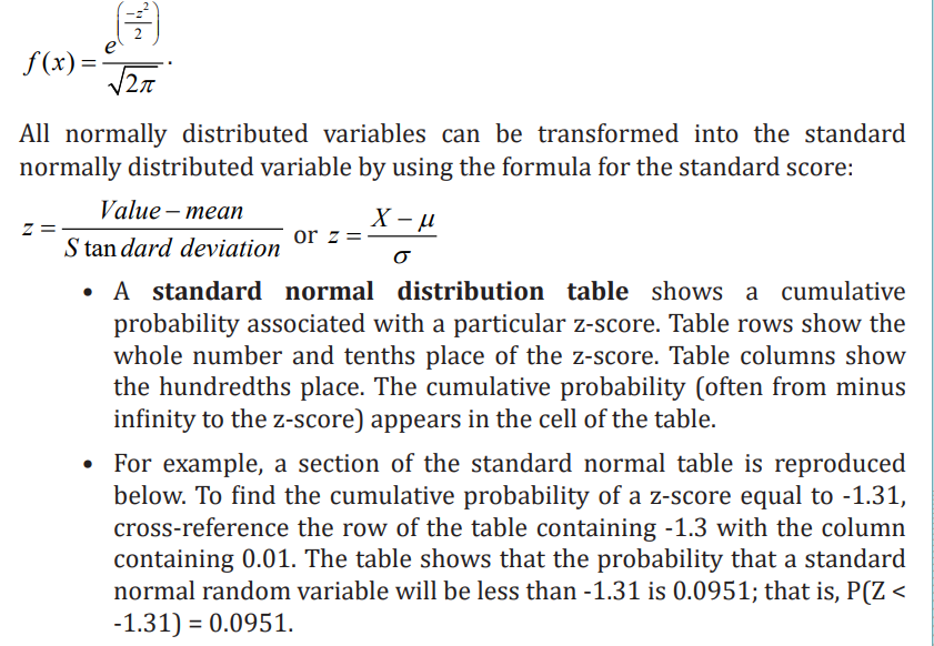
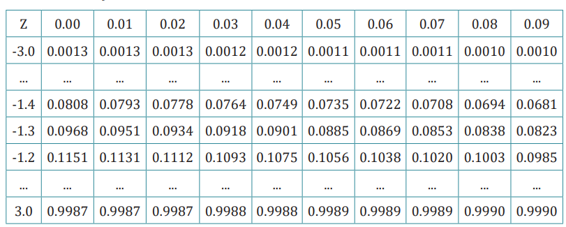
Standard Normal Distribution: A normal distribution in which the mean
is 0 and the standard deviation is 1. It is denoted by z and Z score is used to
represent the standard normal distribution.The formula for the standard normal distribution is
Examples:
1. The age of the subscribers to a newspaper has a normal distribution with
mean 50 years and standard deviation 5 years. Compute the percentage
of subscribers who are less than 40 years old and the percentage of whoare between 40 and 60 years old.
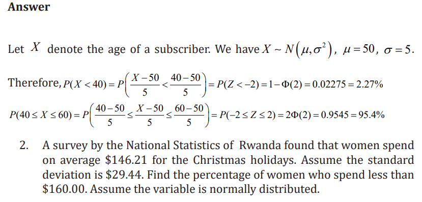
Solution:
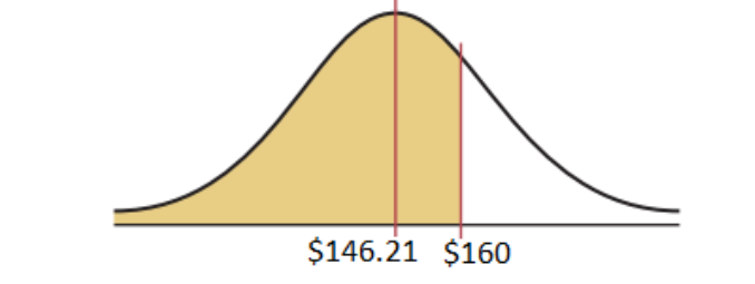
Step 1 Draw the figure and represent the area as shown in the following figure
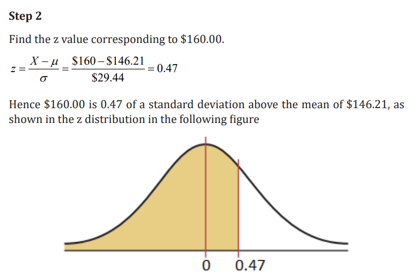
Step 3
Find the area, using the table which is on appendix of this student book. The
area under the curve to the left of z = 0.47 is 0.6808. Therefore 0.6808, or68.08%, of the women spend less than $160.00 at Christmas time.
Application activity 5.2.6
5.3. Applications of probability and probability distributions
in finance, economics, businesses, and production relateddomain.
Learning activity 5.3
1. The Trucks packed goods stayed at MAGERWA for under clearing
process in certain days. The number of days shown in the distribution aredisplayed in the table below:
Find these probabilities: (a) A Truck stayed exactly 5 days. (b) A Truck stayed
less than 6 days. (c) A Truck stayed at most 4 days. (d) A Truck stayed at least5days
Probability is essential in all aspects of human activities. Through this, we
can calculate families welfare, get information on different aspects of life and
planification in order to predict the future. It is very important to incorporate
probability with their properties looking at distributions to adresss these real-world issues. Therefore, probability play a great role for decision makers
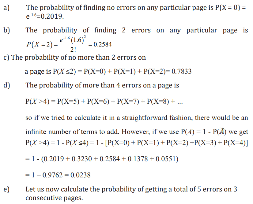
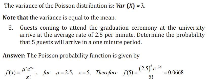
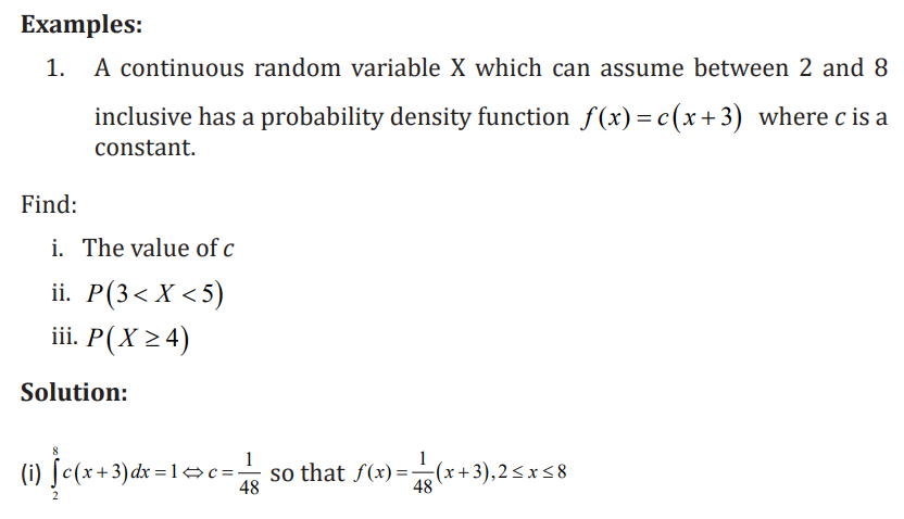
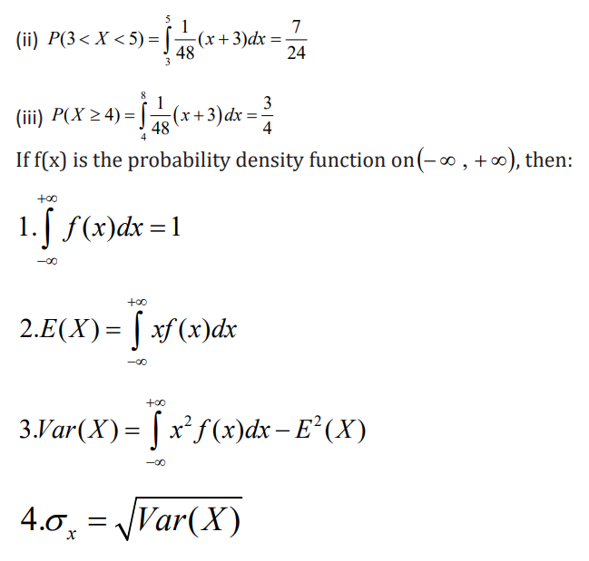
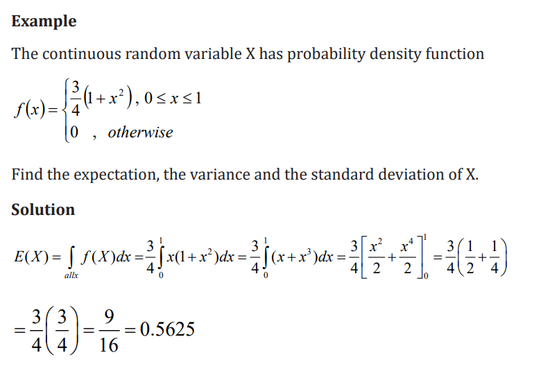
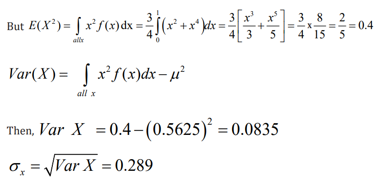
Examples:
1. In Economics, A welfare of families depending on family planning. A woman
planning her family considers the following schemes on the assumption thatboys and girls are equally likely at each delivery:
a) Have three children.
b) Bear children until the first girl is born or until three are born, whichever
is sooner, and then stop.
c) Bear children until there is one of each sex or until there are three,whichever is sooner, and then stop.
there are equal numbers of male and female drivers insured with the
Assurance Association, which selects one of them at random.
a) What is the probability that the selected driver makes a claim this year?
b) What is the probability that the selected driver makes a claim in twoconsecutive years?
c) If the insurance company picks a claimant at random, what is theprobability that this claimant makes another claim in the following year?
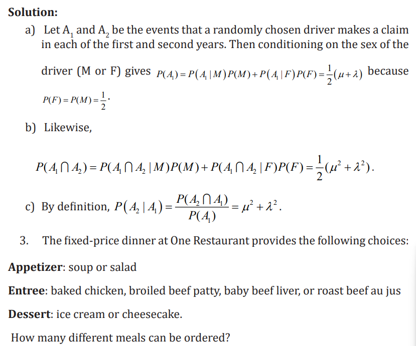
Solution:
Ordering such a meal requires three separate decisions:
Choose an Appetizer: 2 choices. Choose an Entrée: 4 choices. Choose aDessert: 2 choices.
Look at the tree diagram in the following figure. We see that, for each choice of
appetizer, there are 4 choices of entrees. And for each of these 24 8 × = choices,
there are 2 choices for dessert. A total of 2 4 2 16 ××= different meals can beordered.
Application activity 5.3
1. An automatic Shaw machine fills plastic bags with a mixture of
beans, broccoli, and other vegetables. Most of the bags contain
the correct weight, but because of the slight variation in the size
of the beans and other vegetables, a package might be slightly
underweight or overweight. A check of 4000 packages filled in thepast month revealed:
What is the probability that a particular package will be either underweight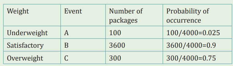
or overweight?
2. A baker must decide how many specialty cakes to bake each morning.
From past experience, she/he knows that the daily demand for
cakes ranges from 0 to 3.Each cake costs $3.00 to produce and
sells for $8.00, and any unsold cakes are thrown in the garbage atthe end of the day.
a) Set up a payoff table to help the baker decide how many cakes tobake
b) Assuming probability of each event is equal, determine the expectedvalue of perfect information.
5.4. End unit assessment
1. Which of the following experiments does not have equally likely
outcomes?
a) Choose a number at random between 1 and 7,
b) Toss a coin,
c) Choose a letter at random from the word SCHOOL,d) None of the above.
2. Tickets numbered 1 to 20 are mixed up and then a ticket is drawn at
random. What is the probability that the ticket drawn has a numberwhich is a multiple of 3 or 5?
3. In a class, there are 15 boys and 10 girls. Three students are
selected at random. What is the probability that 1 girl and 2 boysare selected?
4. One card is drawn at random from a pack of 52 cards. What is the
probability that the card drawn is a face card (Jack, Queen and Kingonly)?
5. The letters of the word FACETIOUS are arranged in a row. Find theprobability that
a) the first 2 letters are consonants,
b) all the vowels are together
6. At a certain school, the probability that a student takes Auditing
and Taxation is 0.087. The probability that a student takes Auditing
is 0.68. What is the probability that a student takes Taxation giventhat the student is taking Auditing?
7. A car dealership is giving away a trip to Akagera National Park to
one of their 120 best customers. In this group, 65 are women, 80
are married and 45 married women. If the winner is married, whatis the probability that it is a woman?
8. For married couples living in a certain suburb the probability that
the husband will vote on a bond referendum is 0.21, the probability
that his wife will vote in the referendum is 0.28, and the probability
that both the husband and wife will vote is 0.15. What is theprobability that
a) at least one member of a married couple will vote ?
b) a wife will vote, given that her husband will vote ?
c) a husband will vote, given that his wife does not vote ?
9. The probability that a patient recovers from a delicate heart
operation is 0.8. What is the probability that
a) exactly 2 of the next 3 patients who have this operation will survive ?
b) all of the next 3 patients who have this operation survive ?
Bibliography
1. Allan G. B. (2007). Elementary statistics: a step by step approach, seventhedition, Von Hoffmann Press, New York.
2. David F. Groebner, (2008),Business Statistics-Decision Making, 7th edition.Prentice Hall.
3. David R. (2000). Higher GCSE Mathematics, revision and Practice. OxfordUniversity Press, UK.
4. David Rayner, Higher GCSE Mathematics, Oxford University Press 2000
5. Douglas A. Lind, William G. Marchal and Robert D. Mason, (2002),
Statistical Techniques in Business & Economics,11th edition, New York,McGraw-Hill Irwin.
6. Frank Ebos, Dennis Hamaguchi, Barbana Morrison & John Klassen,
Mathematics Principles & Process, Nelson Canada A Division ofInternational Thomson Limited 1990
7. Geoff Mannall & Michael Kenwood, Pure Mathematics 2, HeinemannEducational Publishers 1995
8. George B. Thomas, Maurice D. Weir & Joel R. Hass, Thomas’ CalculusTwelfth Edition, Pearson Education, Inc. 2010
9. Gerald Keller, Brian Warrack, (2003), Statistics for Management andEconomics, 6th edition, Duxbury Thomson Learning, Pacific Grove.
10. https://www.brainkart.com. Business mathematics 11th std. cost functionfrom marginal cost function
11. https://www.google.com/search? q=application +of+probability+
in+business&oq=&aqs=chrome. 0.35i39i362l5 j46i39i362j35i39i3
62l2.257365776 j0j15&sourceid = chrome&ie=UTF-8, retrieved 4th, Feb,2024
12. https://www.johndcook.com/blog/forecasting/ , retrieved 4th, Feb 2024
13. J CRAWSHAW, J CHAMBERS: A concise course in A-Level statistics withworked examples, Stanley Thornes (Publishers) LTD, 1984.
14. J. CRAWSHAW and J. CHAMBERS 2001. A concise course in Advanced LevelStatistics with worked examples 4th Edition. Nelson Thornes Ltd, UK.
15. J. Sadler, D. W. S. Thorning: Understanding Pure Mathematics, OxfordUniversity Press 1987.
16. James T. McClave, P. George Benson and Terry Sincich, (2008), Statistics forBusiness and Economics, Prentice Hall.
17. James T. McClave, P.George Benson. Statistics for Business and Economics.USA, Dellen Publishing Company, a division of Macmillan, Inc 1988.
18. James T. McClave, P.George Benson. Statistics for Business and Economics.USA, Dellen Publishing Company, a division of Macmillan, Inc 1988.
19. Jean-Philippe RÉAU and Gérard CHAUVAT, (1999), Probabilités &Statistiques. Armand Colin.
20. John bird. (2005). Basic engineering mathematics. 4th Edition. LinacreHouse, Jordan Hill, Oxford OX2 8DP
21. K.A. Stroud. (2001). Engineering mathematics. 5th Edition. Industrial Press,Inc, New York
22. Ngezahayo E.(2016). Advanced Mathematics for Rwanda secondarySchools, Learners’ book 4, Fountain publishers, Kigali.
23. Ngezahayo E.(2016). Advanced Mathematics for Rwanda secondarySchools, Learners’ book 4, Fountain publishers, Kigali.
24. Ngezahayo E.(2016). Subsidiary Mathematics for Rwanda secondarySchools, Learners’ book 4, Fountain publishers, Kigali.
25. Ngezahayo E.(2017). Advanced Mathematics for Rwanda secondarySchools, Learners’ book 5, Fountain publishers, Kigali.
26. Ngezahayo E.(2017). Subsidiary Mathematics for Rwanda secondarySchools, Learners’ book 5, Fountain publishers, Kigali.
27. Ngezahayo E.(2017). Subsidiary Mathematics for Rwanda secondarySchools, Learners’ book 5, Fountain publishers, Kigali.
28. Ngezahayo E.(2018). Advanced Mathematics for Rwanda secondarySchools, Learners’ book 6, Fountain publishers, Kigali.
29. Ngezahayo E.(2018). Advanced Mathematics for Rwanda secondarySchools, Learners’ book 6, Fountain publishers, Kigali.
30. Norman L. Johnson, Samuel Kotz and Adrienne W. Kemp, (1992). UnivariateDiscrete Distributions, 2nd Edition. John Wiley & Son.
31. Peter S. (2005). Mathematics HL&SL with HL options, Revised edition.Mathematics Publishing PTY. Limited.
32. Peter Smythe: Mathematics HL & SL with HL options, Revised Edition,Mathematics Publishing Pty. Limited, 2005.
33. REB (2020), Mathematics for TTCs year three, Science and MathematicsEducation (SME), Kigali, Rwanda
34. REB (2020), Mathematics for TTCs year three, social studies education(SSE), Kigali, Rwanda
35. REB. (2015). Subsidiary Mathematics Syllabus, MINEDUC, Kigali, Rwanda.
36. REB. (2019). Mathematics Syllabus for TTC-Option of LE, MINEDUC, KigaliRwanda.
37. S. Brown and W. K. Wong, (2015). Probability and Statistics with
Applications in Finance and Economics, Hindawi, The Scientific WorldJournal 2015:618785, DOI: 10.1155/2015/618785, License CC BY
38. Sadler A. J & Thorning D.W. (1997). Understanding Pure mathematics,Oxford university press, UK.
39. Seymour Lipschutz, PhD. & Marc Lipson, PhD. (2007). Discrete mathematics.3rd edition.
40. Seymour Lipschutz. Schaum’s outline of Theory and Problems of FiniteMathematics. New York, Schaum Publisher, 1966
41. Shampiyona Aimable : Mathématiques 6. Kigali, Juin 2005.
42. Wellars Banzi, and Nteziyaremye Stanislas, (2023). Business Research
Methodology and Operations Research Lectures note, Republic of Rwanda,Kigali Independent University.