S4: ICT in Accounting

Introductory activity

Create the following table in a spreadsheet:

 i) Apply borders as done with the table above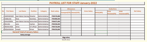
 ii) Enter all data as provided in the table above 
iii) Calculate staff allowances, Gross salary, deductions and Net 

salary

iv) Using SUM, AVERAGE, MAX and MIN, calculate the General 
total of January Salary, Salary average, the staff who gain a big 

salary and the one who get less salary than others.

3.1 Worksheet and workbooks basics

 Activity 3.1

 1. Compare a worksheet and a workbook
 2. Outline 5 features of Ms excel
 3. Using internet search and discuss the following:
 • Amortization of a loan
 • Different steps of creating a loan amortization schedule

Microsoft Excel is one of the spreadsheet programs that helps to store and 
represent data in a tabular form, manage and manipulate data, create optically 
logical charts, and more. 

To open Microsoft Excel, click on the Start button and search for the MS Excel 
application. Double click on the Excel icon to open the Excel. When Excel opens, 

an interface will appear. 

3.1.1. Introduction on workbooks and worksheets

 A workbook is a collection of many sheets. A worksheet is made of rows and 
columns that intersect each other to form cells where data is entered. In Excel 
worksheet, rows are represented by numbers and columns by alphabets.
 
A single Excel workbook can consist of several sheets, named Sheet1, Sheet2, 
Sheet3, etc. One or more sheets can be added to an Excel workbook. By 

clicking to the Plus (+) sign next to a worksheet name.

A. Opening an existing workbook
 An existing Excel file (workbook) is opened in the same way as other files. First 
know where it is located and open the folders where it is stored. When reached 
double click it.

 An existing file can also be opened from an opened Excel file. To do it do the 

following:

 In addition to creating a new workbook. An existing workbook may contain data.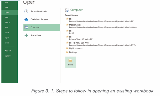 
It can be opened directly from the location where it is stored or through MS 

Excel. Follow the given steps below:

B. Worksheet environment
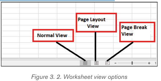
 A worksheet consists of many rows and colums and other tools that are used 
to carry out different operations. When using a worksheet, the user has also to 
be aware of the different views possible which will rule how the worksheet will 
appear. There are three main views namely Normal View, Page Layout View 
and Page Break View. 

The different views are accesses by clicking to their respective icons which are 

located in a worksheet near the bottom left corner.

A worksheet contains different tools which are shown below:

3.1.2. Operations on a worksheet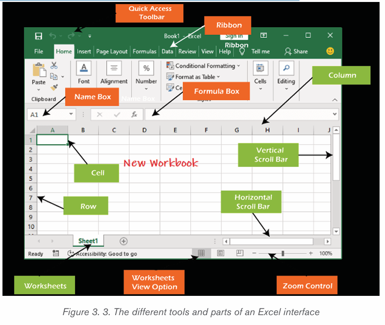
 Excel enables the users to perform several types of operations on Excel 
worksheet and its data. For example, Rename a worksheet, insert a new 
worksheet, delete a worksheet, and many more.

 A. To rename a worksheet
 A new worksheet named Sheet1 gets added to the workbook by default. Excel 
allows its users to rename the worksheet name. A worksheet is renamed in 
order to reflect its content. Follow these steps to rename a worksheet:
 1. Right-click on the worksheet to be renamed, then select Rename from 

the worksheet menu.

2. Type the desired name for the worksheet. In this case «januar» has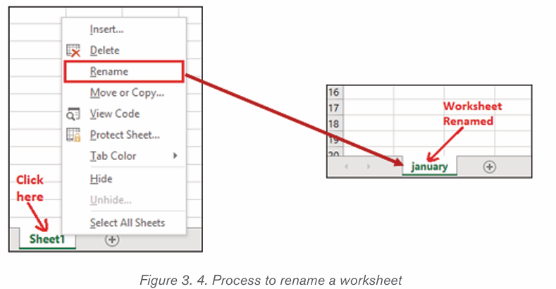 

been written

3.Click anywhere outside of the worksheets, or press the Enteron our keyboard.
The worksheet will be renamed.

B. To create a new worksheet
 Excel provides a new sheet button (+ symbol) near the different worksheet 
names that allow the users to add any number of worksheets to their currently 
active workbook. To create a new worksheet click on that Plus button a new 

worksheet is immediately created

C. To delete a worksheet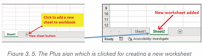
 1. Right-click on the worksheet to be removed then select Delete from 

the worksheet menu.

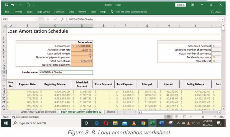
3.1.3. Loan amortization worksheet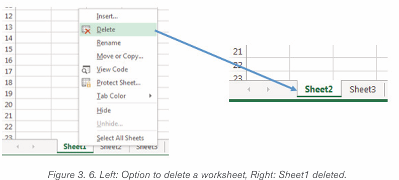 
Loan amortization is the process of scheduling out a fixed-rate loan into equal 
payments. A portion of each installment covers interest and the remaining 

portion goes towards the loan principal.

In banking and finance, an amortizing loan is a loan where the principal of the 
loan is paid down over the life of the loan according to an amortization schedule, 

typically through equal payments.

Creation of loan amortization worksheet
 In order to create an amortization of a given loan follow these steps :
 1. Select the worksheet on which a loan amortization can be calculated. 
2. Right click on the selected worksheet and click on Insert
 3. Click on Spreadsheet solutions on the insert window
 4. The select Loan Amortization

 5. Then click Ok

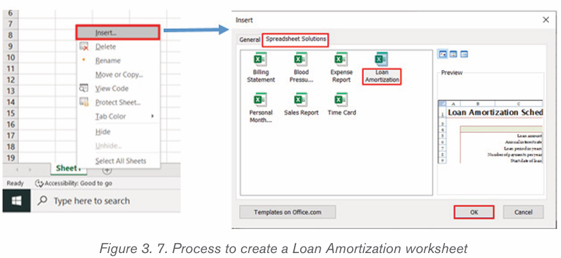
 The loan amortization worksheet will appear like in the window below

Application activity 3.1

 1. UMURAZA Febronie is a secondary teacher at G.S. MUHAMBARA, 
she went to UMWALIMU SACCO to request for a salary advance 
loan of 2000000 Rwf to be payed in three years (36 months) . As 
a loan officer, create a loan Amortization schedule for that teacher.
 
2. Explain how you can :
 a) Add new worksheet 
b) Delete a worksheet

 c) Rename a worksheet

3.2. Cells basics

Activity 3.3

 1. Given the following table created in a Excel:

 a) a. Using cells references, calculate the Total Price for each item and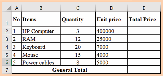
 b) b. The General Total

 3.3.1 Cell references
 There are three types of references in Excel namely relative cell references, 
absolute cell references and mixed cell references in Excel
 
0. Relative Cell References
 By default, all cell references are relative references. Relative references are 
changed when copied across different cells based on the relative positions of 
rows and columns. For example, suppose this formula =B1*C1 is to be copied 

from row 1 to row 2, the formula will become =B2*C2. Relative reference is 

useful when it requires to repeat a calculation across numerous rows or columns.

1. Absolute Cell References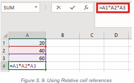
 Absolute cell reference is one in which the cell references being referred to do 
not change like they did in a relative reference. To set an absolute cell reference 
use the $ sign by pressing f4 to create a formula for absolute referencing. The $ 
sign means lock, and it locks the cell reference for all of the formulas, ensuring 
that the same cell is referred to all of them. To use a formula with absolute cell 
reference use the $ (dollar sign) in front of every cell.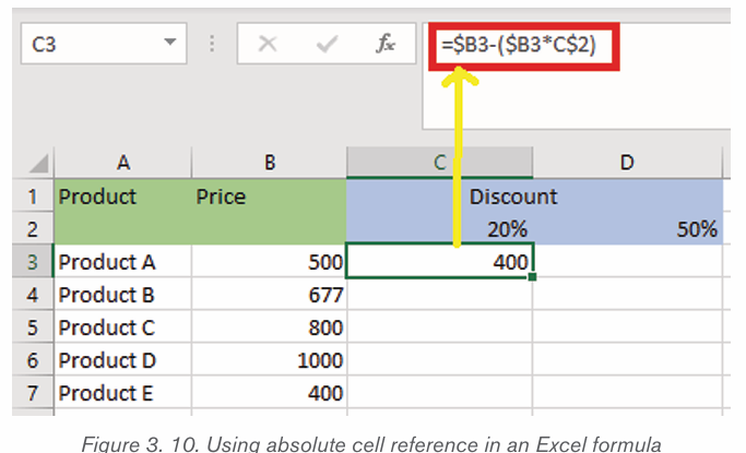

 
2. Mixed Cell Reference in Excel
 A Mixed cell reference is a mixture of both relative and absolute cell reference. In 
mixed cell reference, dollar signs are attached to either the letter or the number. 
For example, $B2 or B$4. It’s a mix of relative as well as absolute reference.

There are two types of mixed cell references:
 1. The row is locked while the column changes when the formula is copied.
 2. The column is locked while the column changes when the formula is 

copied.

3.3.2 Text Alignment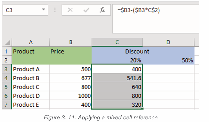 
Text alignment is a feature that helps users to align text within worksheet cells. 
It enables the composition of text documents with various text positions or 
alignments on one or more cells within the Excel document. 

a. Change Text Alignments from Ribbon
 The easiest and straightforward way to access text alignment options in 
Excel is to use ribbon tools. Both horizontal and vertical alignment options 
can be accessed by going to the Home tab and using the alignments from 

the Alignment group.

By default, Excel automatically aligns entered text contents to the left position of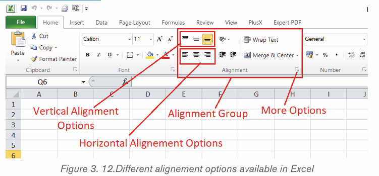 
the cell and numbers to the right position. Alignment options from the Alignment 
group can be used to change the alignment accordingly.
 
Follow these steps to align a text:
 • Select the text to be aligned
 • Click the tool to be used from the vertical alignment options and pick 
Top Align, Middle Align, or Bottom Align, respectively.
 • Click the tools from the horizontal alignment options and pick Left Align, 
Center Align, or Right Align, respectively.
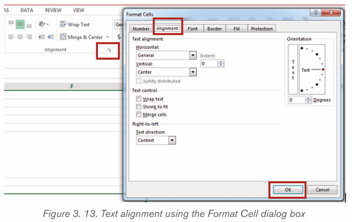
 a) Change Text Alignments from Format Cells
 
The Format Cells dialog box is another efficient way to change text alignments 
in Excel cells. Perform the following steps to use this method:
 • First, select the cells on which to align texts.
 • Open a Format Cells dialogue box and launch a dialogue box by 
clicking the arrow at the bottom right corner of the Alignment group 
under the Home tab.
 • In the new dialog box that appears click on Alignment
• Select the different types of alignment to be applied. If the text orientation 
needs to be changed change it using the Orientation option which is 
set by moving the needle or setting the text orientation degrees.

• Click on OK to apply the new text alignment

Alternately, pressing Ctrl+1 the keyboard shortcut keys combination can open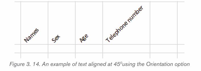 

the Format Cells dialogue box.

 3.3.3 Setting Font
 Excel has a variety of built-in customizations that can help to change the 
appearance of the sheet to a maximum extent. The font properties that can be 
changed are: font type, font size, font color, and changing the text to bold, Italc 
and Undelining the text. The font can be changed using the menu Ribbon or 

using the Format Cells dialog box.

 • Changing Font Type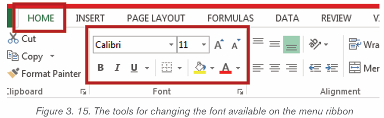
 To change the font type or style using the menu ribbon in one or more Excel 
cells, perform the following steps:
 • Select the cell (s) consisting of the needed values to format.
 • Next, go to the Home tab and click the initial drop-down list under the 

category font, as shown below :

• We can scroll down to view all the installed fonts on computer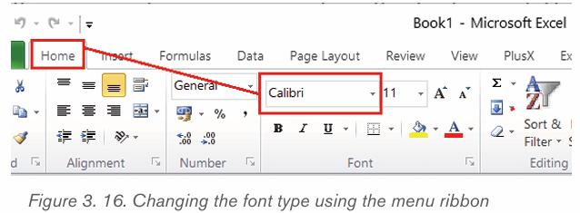 click on 
the desired font type/style to instantly use it in the selected cell (s).
 
• Changing Font Size
 To change the font size in the desired Excel cells, perform the following steps:
 • Select the cells to adjust font size.
 • Go to the Home tab and click on the drop-down list associated with 
the number (i.e., 11, 12, etc.), next to the Font drop-down list, under 

the Category Fonts, as shown below:

 There is a selection of multiple pre-defined font sizes to choose from. to use the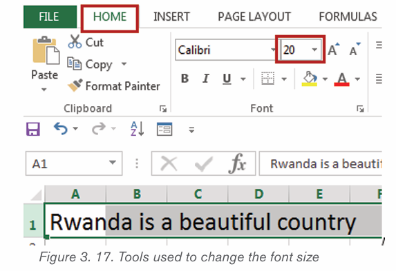 
desired font size, click the number from the list. However, if there is no suitable 
size, type the number directly in the font size box and press the Enter key. 
The font size can be quickly adjusted by clicking on Increase Font Size and 

Decrease Font size tools, displayed next to the Font size box.

 • Changing Font Color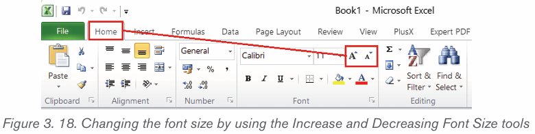
 To change the font color for the desired Excel cells, perform the following steps:
 • Select Excel cells to apply the desired color.
 • Next, navigate the Home tab and click the last drop-down list under 
the category Font. It is associated with the letter ‹A› and a red color bar 

below it. Refer to the screenshot below:

 • After clicking the drop-down arrow for the font color, click on the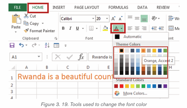 
desired color from the list of Theme Colors or the Standard Colors. 
In this case the red color was clicked.
 
Note: If the cell is empty while setting the font in Excel, then as soon as we start 
typing text or data in the respective cell, the applied style, size, color, etc., will 
be applied automatically.
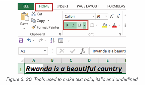
 • Setting Font to use Bold, Italic, and Underline
 
To change the font format in the desired Excel cell to make it bold, italic, or 
underlined, perform the following steps:
 • Select one or more Excel cells to modify their respective values.
 • Go to the Home tab and click the Bold (B), Italic (I), or Underline 
(U) shortcut under the category Font. These tools help to change the 
appearance of the selected cell accordingly. Now the text becomes 

more black, underlined and oblique (italic)

Application activity 3.2

 1. Discuss the different ways of text alignment
 2. Using the data of an Activity 3.2, apply the follwing :
 a. Align on top the first row 
b. Make all items centered 
c. Make the Total Price centered to the right side and make it be in 
a red color
 d. Make the font size of General Total be 18 
e. The font style should be Tahoma, Bold and Italic 
f. Fill the whole table with green color

3.3 Arithmetic operators in formula
 Activity 3.3
1. What do you understand by an operator ?
 2. Give two examples of arithmetic operators and its uses

 In mathematics, the term   operator refers to a sign or symbol used to evaluate 

mathematical operation. 

The most basic mathematical signs are the arithmetic operators which include 

addition (+), subtraction (-), multiplication (×), and division (÷). 

In mathematical computing, the same operators are used but multiplication and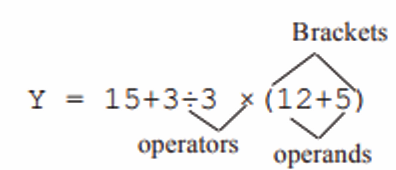 

division operators are replaced with asterisk (*) and forward slash (/) respectively.

The table below, gives a summary of the four arithmetic operators supported in 

Excel and their functions :

3.3.1 Addition operator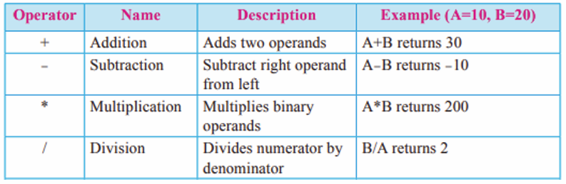 
The addition operator (+) evaluates mathematical addition operation
 Example: The figure below represents data of students ‘performance in three 

subjects. Find the total marks for every student

 To complete the total column, consider the below steps: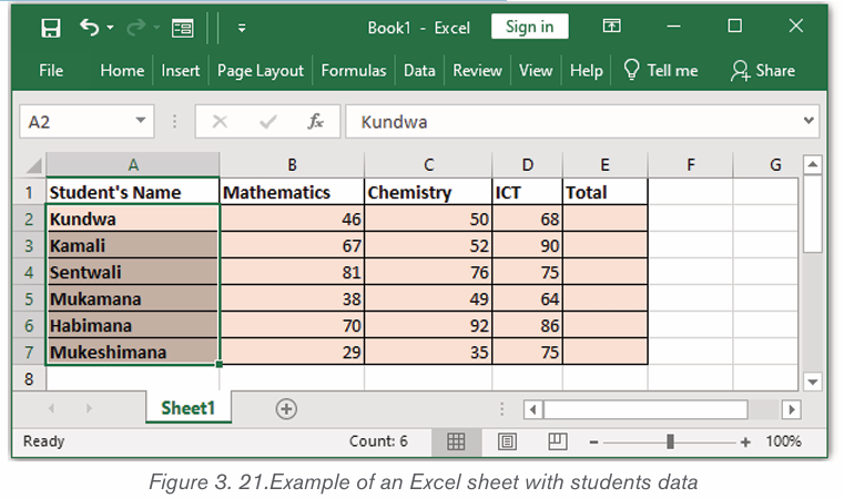
 a. Click on the first cell of the total column.
 b. Drag the mouse on the formula bar and type =B2+C2+D2
 c. Click on the bottom-right corner of that block and drag to the last cell of 
the total column.
 d. And release the mouse, the result will appear on all the specified cells of 

the column as it is shown below:

 3.3.2 Subtraction operator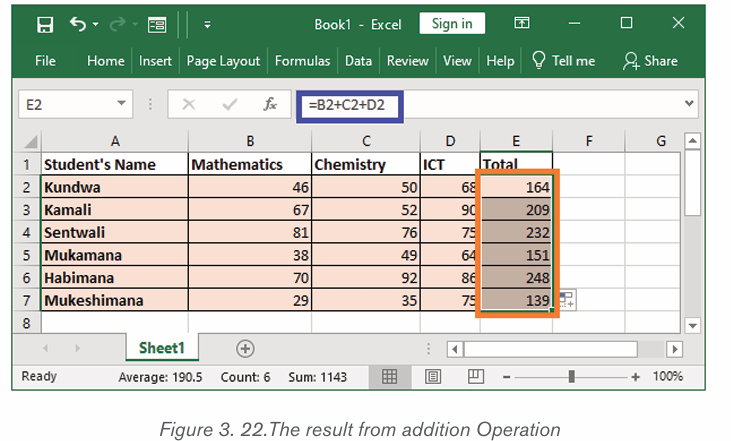 
The subtraction operator (-) evaluates mathematical subtraction operation
 Example: Using data stated in example above, Calculate the difference between 
Mathematics marks for Kundwa and Kamali.
 Perform the following steps:

 a.Click on the cell where the difference/resultat will appear.
b.. Write in cell the Substraction formulas =B3-B2
c. click on enter button, the result will come in cell as it is shown bellow: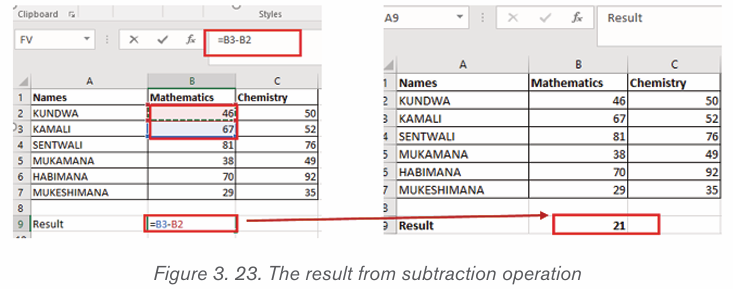

 
3.3.3 Multiplication operator (*)
 The product of numeric values is performed by using a multiplication operator 
in formulas. Let’s use the example of purchasing different products, where the 
total price as product will be obtained by multiplying quantity with price per unit
 Here below, are the steps to be followed:
 
a. Click on the first cell of the Product column.
 b. Drag the mouse on the formula bar and type =B2*C2
 c. Click on the bottom-right corner of that block and drag to the last cell of 
     the Product column

 d. Release the mouse Button, to see the result as follows :

The division operator is used in calculation of quotient of two numeric values.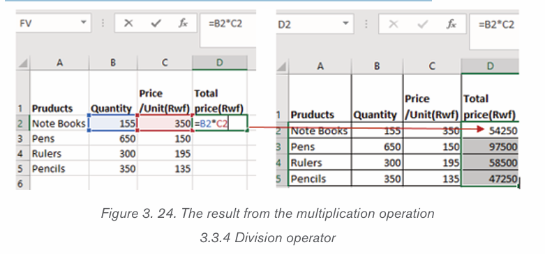  
Use the same data of additional operator in order to understand how division 
operator works.
 For example, let divide total marks for Sentwali by 2. Proceed as follows:
 a. Select F4 cell of the Quotient column.
 b. Drag the mouse on the formula bar and type =E4/2
 c. Press Enter key to find the result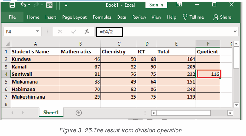

Application activity 3.3
1. Study the figure given below that presents   the national examination 

result of 4 primary students and wok out the related questions 

a) Calculate the total marks for all given students. Total marks will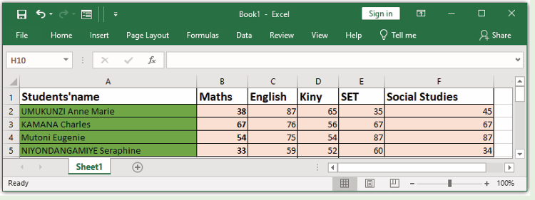 
appear in G column 
b) Calculate the difference between the marks of UMUKUNZI and MUTONI
 c) The marks of mentioned students are on 100 for each subject. 
You are requested to put their total marks on 100. The result will 
appear in H column. 
d) For each student, add 2marks on her/his percentage of marks
 e) For student named NIYONDANGAMIYE, add 3marks to each subject
 
3.4. The use of functions 
Activity 3.4
 After doing a research on internet or any other resource:
 a. Identify different parts of a function
 b. Explain different types of functions available in 

Excel.

3.5.1 The parts of a function
 In order to work correctly, a function must be written in a specific way. The 
basic syntax for a function is the equals sign (=) followed by the function 
name (SUM, for example), and one or more arguments. Arguments contain 
they are numbers or any other data on which the function operations are going 
to be done. The arguments of a function can be written in two ways:
 • Writing every single argument in a function. This option is used when 
the arguments to be added are not many.
 • Writing the range starting from the first argument to the last argument. 
This is possible only if the cells (arguments) are in the same row or in 

the same column. 

 Arguments can refer to both individual cells and cell ranges and must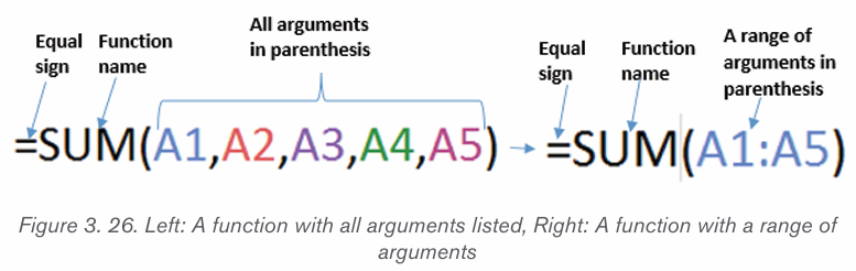 
be enclosed within parentheses. You can include one argument or multiple 
arguments. 
 
3.5.2 Excel Aggregate functions

 A  SUM function

The sum SUM function is used to add numbers. It can add two or more arguments 
which are all enclosed in parenthesis or just a range of arguments starting from 
the first cell and ending by the last cell. In the first case, cells (arguments) are 
separated by comma (,) while for the second case the first and last cell are 

separated by a colon (.

 For example the function =SUM(A2,B2,C2,D2,E2) will add the values of in the 
cells A2,B2,C2,D2 which are in the same row. This same function can 

be written as =SUM(A2:E2).

 To use the SUM function and get addition results like in the screenshot above,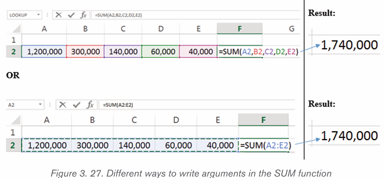 
do the following:
 • Put the cursor in the cell where the sum will be calculated and write an 
Equal sign (=)
 • Write the word SUM and put the cursor inside the parentheses
 • If all the cells (arguments) will appear in the parentheses, click on every 
call and write a comma after every cell. If only the first cell and the last 
will appear in the parentheses just select all the cells whose content is 
to be added
 • Click outside the cells for the sum to be calculated

 When the data to be added is not in the same row or the same column, 
the two ways of writing arguments can be used. For example, the function 
=SUM(A1:A3,C1:C2,E1) will add the values of all of the cells A1 to A3 then C1 

to C2 and E1. This same function can be written as =SUM(A1,A2,A3,C1,C2,E1)

The AutoSum command allows you to automatically use the most common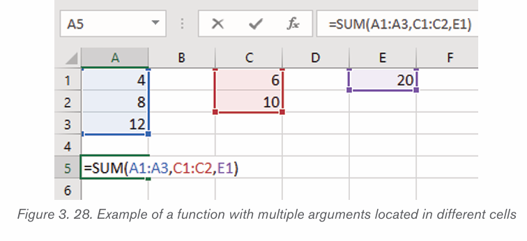 
functions including SUM, AVERAGE, COUNT, MIN, and MAX. In the example 
below, the SUM function is accesses by using the AutoSum command. The 
AutoSum command is available under the Formula tab. It can also be accessed 
under the Home tab in the Editing group.

1. Select the cell that will contain the function. 
2. In the Editing group on the Home tab, click the arrow next to 
the AutoSum command. Next, choose the desired function from the 

drop-down menu. In this example Sum was selected.

1. Excel will place the function in the cell and automatically select a cell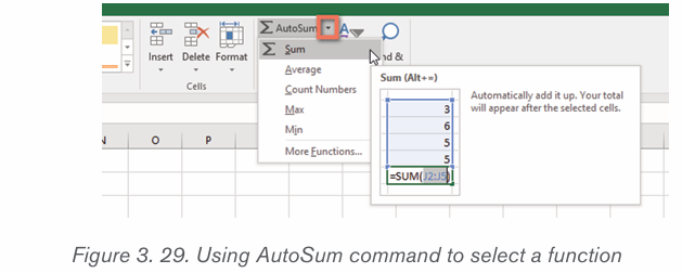 
range for the argument. In this example, cells D2:D7 were selected 
automatically; their values will be added to calculate the total cost. If 
Excel selects the wrong cell range, you can manually enter the desired 
cells into the argument.
 
2. Press Enter on your keyboard. The function will be calculated, and 

the result will appear in the cell. 

B. AVERAGE function

The average function determines the average of the values included in the 
argument. It calculates the sum of the cells and then divides that value by the 
number of cells in the argument. 
Its syntax if all the arguments will appear in the parentheses is:

 =AVERAGE(number1, number2,…) 

 A syntax containing only the first and last cell between the parenteses can also 

be use.

For example, the function =AVERAGE(F1,F2,F3,F4) would calculate 
the average of the values in the cells F1, F2, F3 and F4. This same function 

can also be written as =AVERAGE(F1:F4) 

 To calculate the average using the AVERAGE function as it was done in the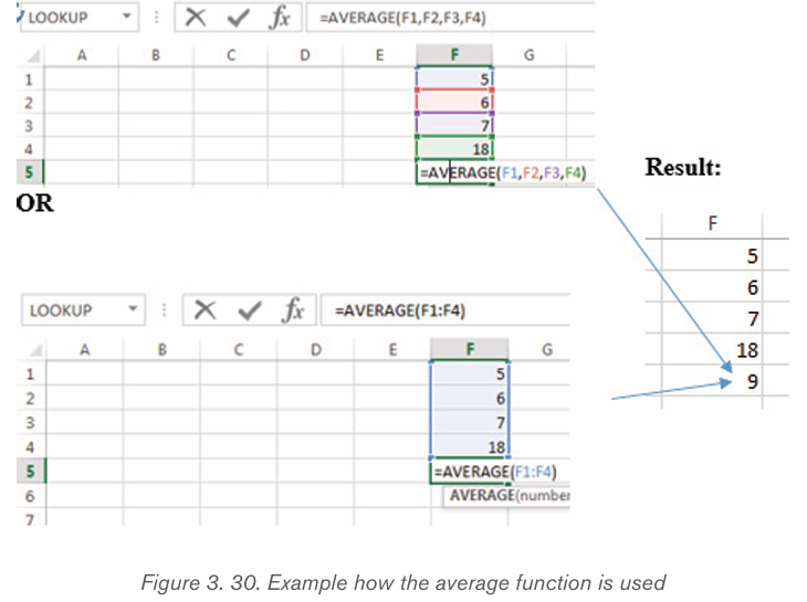 
screenshot above, do the following:

3. Select the cell that will contain the function result. 
4. Type the equals sign (=), and write the function name which is 
AVERAGE. You can also select the desired function from the list 
of suggested functions that appears below the cell as you type.
 5. Enter the cell range for the argument inside parentheses. In this 
example type (F1:F4) or type (F1,F2,F3,F4) or just select those cells.

 Press Enter on the keyboard or click in any other cell. 
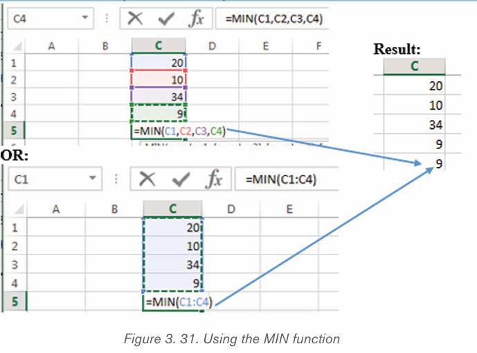
C MIN function
 
The Excel MIN function returns the smallest numeric value in the data provided. 
The MIN function ignores empty cells, the logical values TRUE and FALSE, and 
text values. 

The syntax of the MIN function is:

=MIN(number,number2, …)

This syntax can also be written in such a way that only the first argument (cell) 
and the last appear in the parentheses. In this case, the two cells are separated 

by colon (

Example: =MIN(A1,A2,A3,A4) OR =MIN(A1:A4)
 To use the MIN function proceed in this way:
 • Go in the cell where the min will be calculated 
• Write the Equal sign followed by MIN
 • In the parenteses write the arguments or select them. In this case the 
argments are C1, C2, C3 and C4.

 • Hit the Enter key or click in any other cell for the result to be calculated

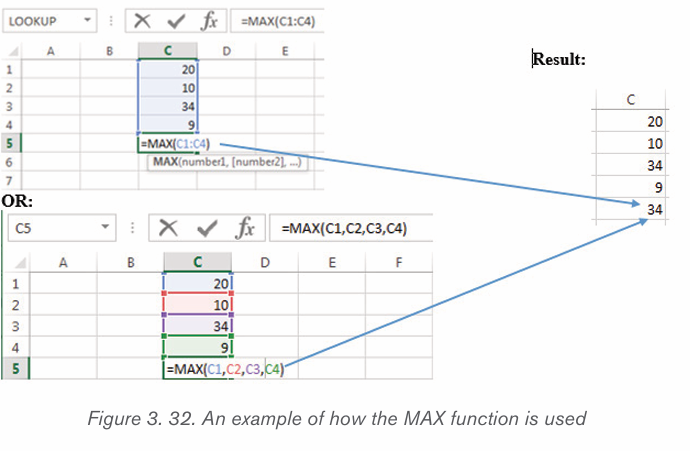
D MAX function

 The MAX function returns the largest numeric value in the data provided. For 
example, MAX function can return the highest marks for a student for all subjects 

or the highest mark for a student for a given subject.

The syntax of the MAX function is:

=MAX(number1,number2,…)
 The arguments in the parentheses can be only the starting cell (argument) and 
the last cell separated by a colon.

 To use the MAX formula in Spreadsheet follow these steps:

6. In a cell where the maximum value will appear, type =MAX
7. Inside the parentheses write the cells for which the maximum number is 
to be calculated or select those cells

 8. Press the Enter key or click in any other cell.

E. COUNT function

 The COUNT function counts the number of cells with numerical data in the 
argument. This function is useful for quickly counting items in a cell range. For 
example, you can enter the following formula to count the numbers in the range 
A1:A20
 
The syntax of the COUNT function is:
 =COUNT(value1,value2,…)
 However there is no need to put in the parentheses all the arguments if the cells 
whose values are to be counted are in the same row or column. 
Use the COUNT function in the following way:
 • Click in the the cell where the count value will appear and type 
=COUNT
 • Inside the parentheses write the cells that will be counted
 • Press the Enter key or click in any other cell.
 Note that the COUNT function does not consider cells with content other that 

numbers. It does not consider text or empty cells.

Note that in the second screenshot the result of the COUNT function is 4 instead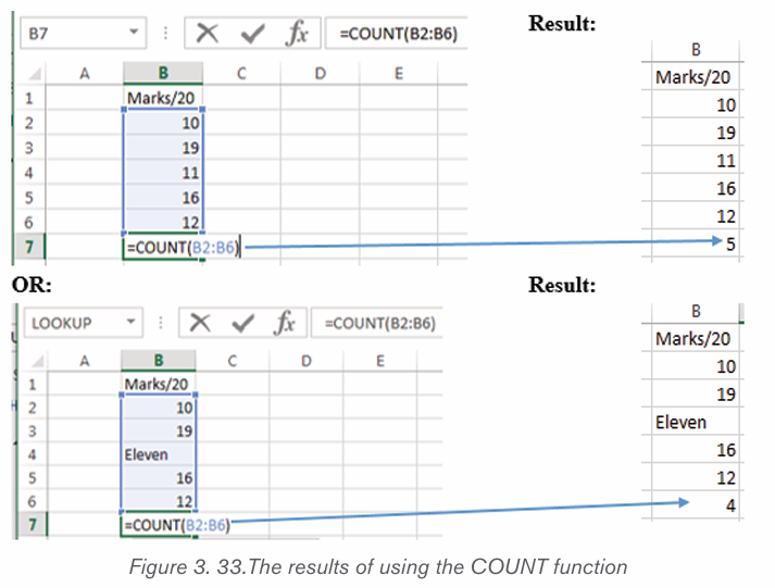 

of being 5. This is because this function does not count cells containing text.

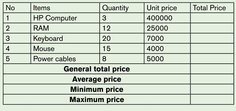
Application activity 3.5

Types the following and then calculate the total price, general total, average, 

minimum and maximum using spreadsheet functions

3.5. Tables and borders design

 Activity 3.5

 a) What do you understand by table borders?
 b) With internet search ,
 c) 1) Explain the importance's of using tables borders 

d) Discuss different steps of applying borders

 In Excel, borders refer to a line drawn across any or all of four sides of a cell in 
a worksheet. When adding a border to one or more cells, choose specific sides 
to include or exclude. Moreover, borders for custom or desired sides of cells 
can be drawn manually. 

• Applying borders from ribbon
 Excel Ribbon is the primary area for accessing most existing commands or tools. 
While creating a border in Excel, we can take advantage of the Excel ribbon and 
apply a border to the desired cell using the following steps:
 • Select the Excel cells on which to apply borders. Hold down the 
mouse›s left button and drag the selected shading from one cell to the 
others. When selecting non-adjacent cells in Excel, click on individual 
cells while holding down the Ctrl key.
 • Go to the Home tab on the ribbon and click on the drop-down icon 
next to Border
 • Click on the desired border style to apply it. Here All Borders was 

selected.

 Although there are many existing border options, sometimes, borders can be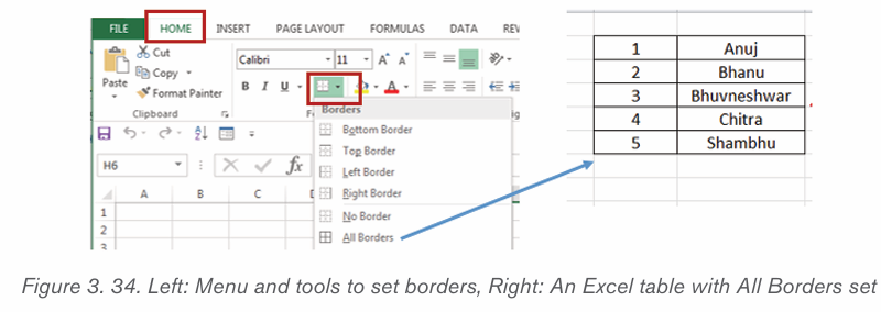 
drawn using the Draw Border option from the drop-down list. This option is 
accesses after clicking on Home then on the Border tool found in the Font 
group. One can also use the Draw Border Grid which create a table over the 

cells moves on.

 A border can be applied using the Format Cells dialog box. Go through the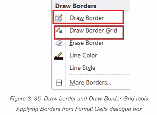 
following steps to access the Format Cells dialog box and insert a border in 
the desired Excel cell:
 • Select the cells in the worksheet.
 • Launch the Format Cells dialogue box by doing a Right click then 
choose Format Cells

 • In the Format Cells dialog box that appears click on Borders 

 • Click on the different border styles to apply then click OK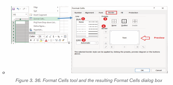

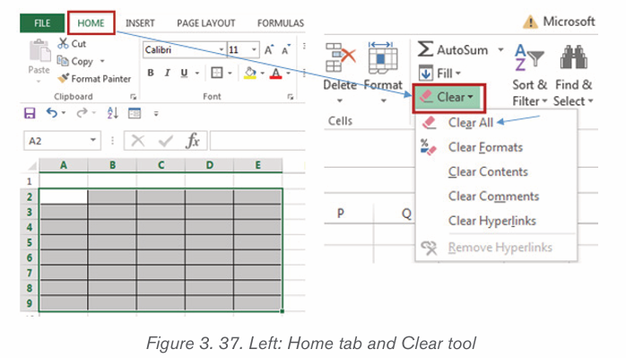
 • Removing borders in Excel
 To remove borders in the Excel worksheet, one of the following methods can 
be used:
 
• Select the cells from which the borders are going to be . Click on Home 

tab then on Border then on No Border.

• To delete borders using the Erase border tool. For this, go to Home 
then click on the Border tool then click on Erase Border. This 
will convert the mouse cursor into an eraser icon, using it erase or 
delete the desired border in the worksheet.

 • Another method is: Select the cells and go to Home then Clear then 
Clear All. Although this method helps remove borders, it also removes 

other formattings like font color, background color, etc. 

Application activity 3.5

 1. Outline differents steps to delete borders
 2. Create the following table and apply the different types borders as 

indicated below:

3.6. Creation of charts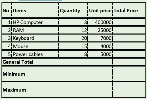
 Activity 3.6
 a. Identify different types of charts you know
 b. Give the importance of using chart for data presentation

 

Charts allow you to illustrate workbook data graphically, which makes it 
easy to visualize comparisons and trends. The data represented through 
charts is more understandable than the data stored in an Excel table. This 
makes the process of analyzing data fast. 

A chart is often called a graph. It bring more understanding to the data 
than just looking at the numbers. Excel offers many charts to represent the 
data in different manners, such as Column Chart, Line Chart, Bar Chart, Area 
chart, Pie Chart
 
To illustrate the different types of charts, the data used are those on a company 
owning a small business of making different types of soap. The quantites of 

soaps in Tons made per year is shown in the table below:

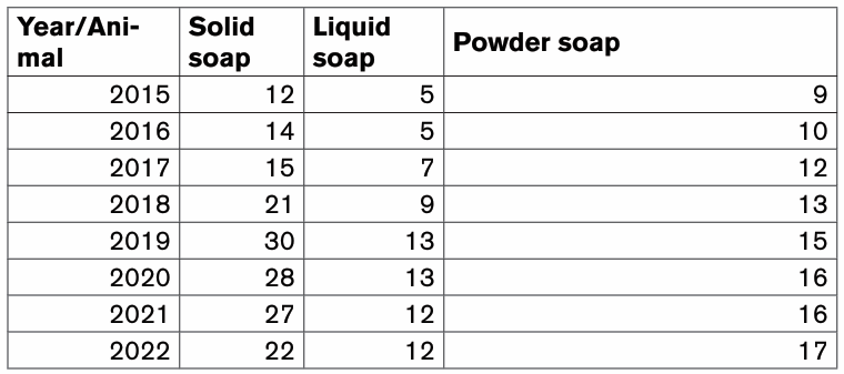
The different charts are inserted by following this procedure:

 • Select the data then click on Insert
• In the Chart group choose one type of chart to be generated. If 
among the visible templates the one needed is not available, click on 

the See All Charts tool to view more chart types

A.Column Charts
 A column chart is basically a vertical chart that is used to represent the data 
in vertical bars. It works efficiently with different types of data, but it is usually 

used for comparing the information.

For example, the company wants to see whose data was shown above wants 
to visualize its production progress from 2015 to 2022 using a column chart. To 
make that column chart the following steps will be used:.
 
Step1: Select the data for which the chart is to be made
 Step 2: On the Insert tab, in the Charts group, choose the type of chart 
to use. In this case the type chosen is the Column chart. Click the 

Column chart symbol

 Step 4: Customize different settings of the created chart by changing the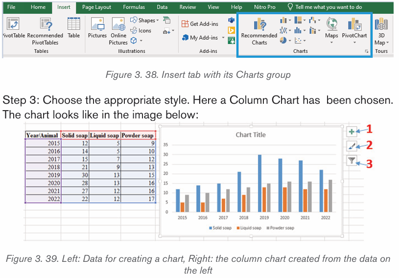 
default chart title (Chart Title) and other settings which are done using the tools 
labelled 1, 2 and 3. The tool 1 is used to add and edit charts elements, the tool 
2 is used to choose any other variant of the chosen chart and the tool 3 is used 

to remove the charts elements that are not needed.

• Adding chart elements
 The chart for can be customized by adding new charts elements. Charts elements 
can be added by clicking on the tool which is labelled as 1 in the above chart. 
The chart below has been customized in order to add the Axis Titles, Data 
labels. The different chart elements are added by ticking the corresponding 

checkboxes.

 • Changing the chart style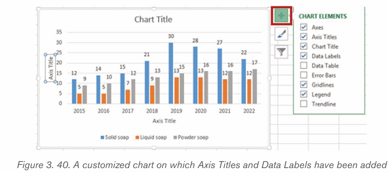 
There are different types of chart which can be used depending on the 
data to display. Switching from one chart type to another is done in this way:
 Step 1: Select the chart for which the type is to be changed
 Step 2: Click on the Chart Styles tool
 Step 3: Click on the new chart type. In this case the chart labelled with an arrow 

was selected.

 Apart from these operations, one can add new elements or remove them using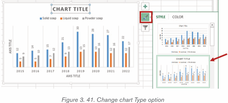 

the Chart Filters option allow to add or remove chart elements like Chart series.

 A. Line Chart
 Line charts are most useful for showing trends. Using this chart, you can easily 
analyze the ups and downs in data over time. In this chart, data points are 

connected with lines.

With the company’s data, a line chart showing the status of the quantities of 
soap produced can be created like by following this procedure:
 • Select the data for which the chart is to be created
 • Click on the Insert tab 
• In the Charts group click on one type of chart here click on the Line Chart

Next to the line chart above there are three tools which are used to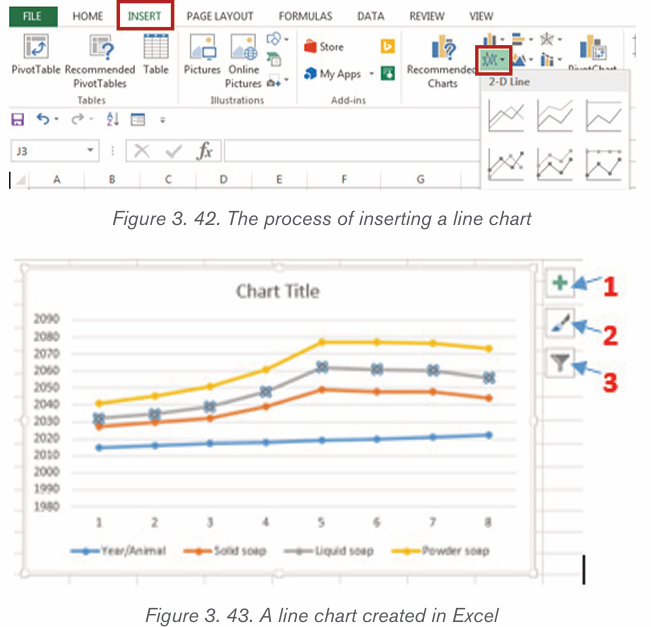 
edit it namely has s tools next to it which are used the Chart Element 
tool (1), the Chart Styles tool and the Chart filters tool.
 
A.Bar chart
 Bar charts are horizontal bars that work like column charts. Unlike column charts, 
Bar charts are horizontally plotted. Or you can say that bar charts and column 
charts are just opposite to each other.
 
The data used in creating line chart and column chard can generate the bar 

chart below:

The chart above was obtained by using the same procedure as for other charts.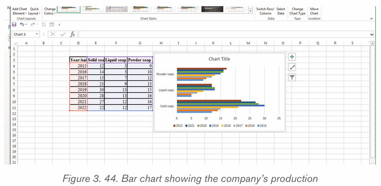 
This procedure involves clicking the INSERT tab then click on the type of chart 
which is now the bar chart and finally selecting the variant of the chart to be 
applied. This chart can be edited using the tools on its left which are Charts 

Elements, Chart Styles, Chart Filters.

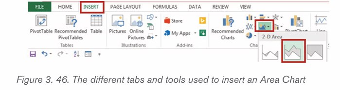
A. Area chart
 Area charts are just like line charts. Unlike the line charts, gaps are filled with 
color in area charts. They are easy to analyze the growth in business as its 
shows ups and downs through line. Information in an area chart is plotted on 
the x and y axis; data values are plotted using data points that are connected 

using line segments.

The data that was used to create the different charts generate the chart below:

The chart above was created by first selecting the data then clicking on the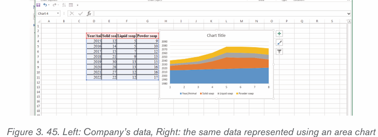 
Insert tab then click on on the Area Chart and then choosing one type of chart 

to use. In the screenshot below, the area chart use is in a red rectangle.

 A. Pie chart

A pie chart is a rounded shape graph that is divided into slices of pie. Using this 
chart, you can easily analyze data that is divided into slices. It makes the data 

easy to compare the proportion.

Like other charts, a pie chart is inserted by selecting the data then clicking on 
the Insert tab and choosing the type of chart which is the Pie chart. This process 

is shown below:

The generated chart lacks some details to be easily understood. That is why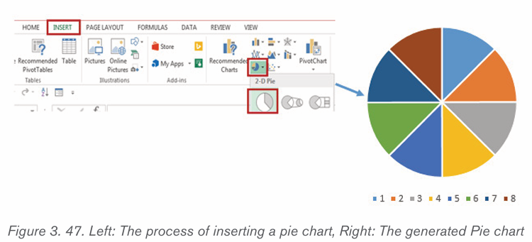 
details can be used by using the Charts Elements, Chart Styles and Chart 
Filters tools. To add those details just click on the tool and check the detail to 

appear on the chart.

The different chart tools shown above can be used to change other charts of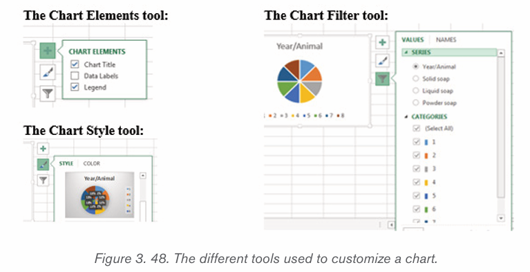 

the same category like the ones shown below:

Application activity 3.6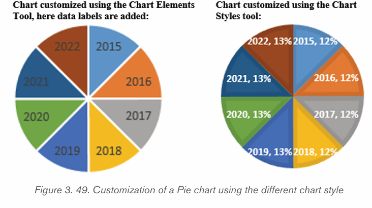
1. Use the following table to create :
 • Line chart
 • Column chart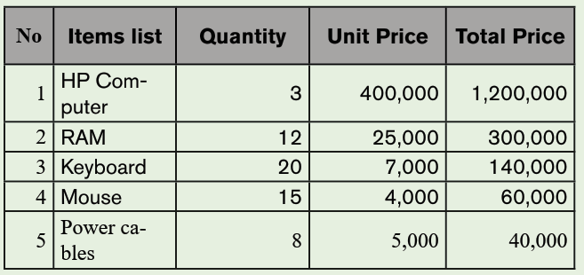

 3.7. Data organization
Activity 3.7
By doing a research using the internet or any other resource
 a. Discuss the types of sorting.
 b. Outline different steps of sorting list in ascending order
 c. What do you understand by filtering data?
After data has been entered into an Excel worksheet and even after it has been 
organized into a table, it can still be manipulated and reorganized. One of the 
easiest options is to sort data in a particular order for example, sorting data 
in alphabetical order. On the other hand, Filtering data allows to analyze data 
easily. When data is filtered, only rows that meet the filter criteria is going to 
 be displayed and other rows will be hidden. Filters narrow down the data in a 
worksheet, allowing to view only needed information.
3.7.1. Filtering data 
After entering data in Excel, it is also possible to filter, or hide some parts of the 
data, based on user-indicated criteria. When using the Filter option, no data is 
lost; it is just hidden from view. 
In order for filtering to work correctly, the worksheet should include a header 
row which is used to identify the name of each column and is used for filtering. 
Follow these steps for filtering data in an excel table:
Step 1: Select the Data tab, and then click the Filter command. Immediately 
a drop-down arrow will appear in the header cell for each column. The filter 
command can also be accessed  by clicking the Home tab and finding it at the far
right side of the menu in the Editing Group.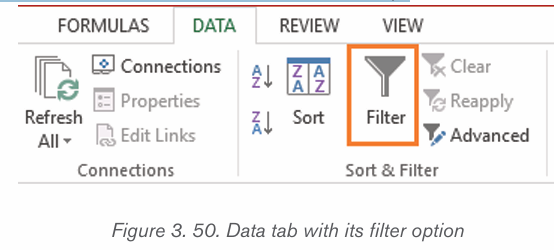

Step 2: Click the drop-down arrow for the column you want to filter. In this 
activity, filter column B (Region) is filtered to view only certain region.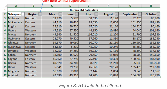

 Step 3: In the Filter menu that will appear uncheck the box next to Select All to 
quickly deselect all data. When the Select All checkbox is unchecked, all the 
other checkboxes will also be unchecked.
Step 4: Check the boxes next to the data you want to filter, and then click OK.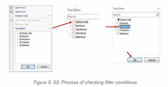

 In this example, Northern is checked to view only those types of equipment 
matching the criteris. The data will be filtered, temporarily hiding any content 
that doesn’t match the criteria.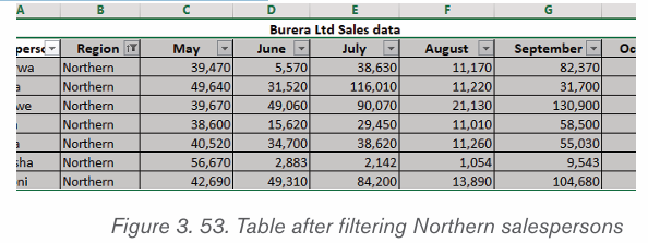

 3.7.2. Clear a filter
 After applying a filter, you may want to remove or clear it from your worksheet so 
you’ll be able to filter content in different ways.
 Step 1: Click the drop-down arrow for the filter you want to clear the Filter 
menu will appear.
 Step 2: Choose Clear Filter from [COLUMN NAME] from the Filter menu. In 
this case the option Clear Filter from «Region» is selected


Step 3: The filter will be cleared from the column. The previously hidden data 
will be displayed like the data was before applying the filter.
 
3.7.3. Sorting 
Sorting refers to ordering data in an increasing or decreasing fashion according 
to some linear relationship among the data items. Sorting can be done on 

names, numbers and records.

Below are steps to sort data:

Step 1: Select the entire table you want to sort
 Note: In most cases, you can select just one cell and Excel will pick the rest 
of the data automatically, but this is an error-prone approach, especially when 

there are some gaps (blank cells) within the data.

 Note: If the first dropdown is showing column letters instead of headings, tick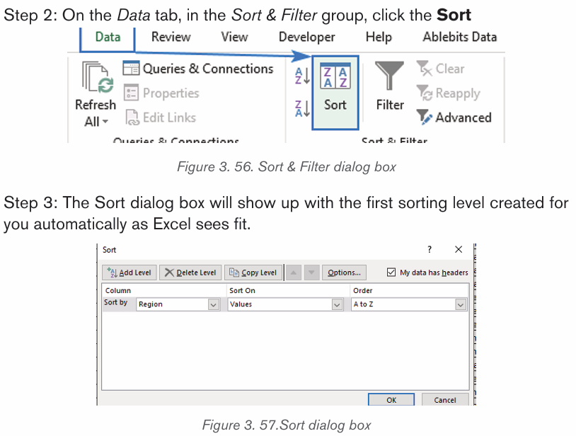 
off the “My data has headers” box.
 
Step 4: Click the Add Level button to add the next level and select the options 

for another column.

 Note: If you are sorting by multiple columns with the same criteria, click Copy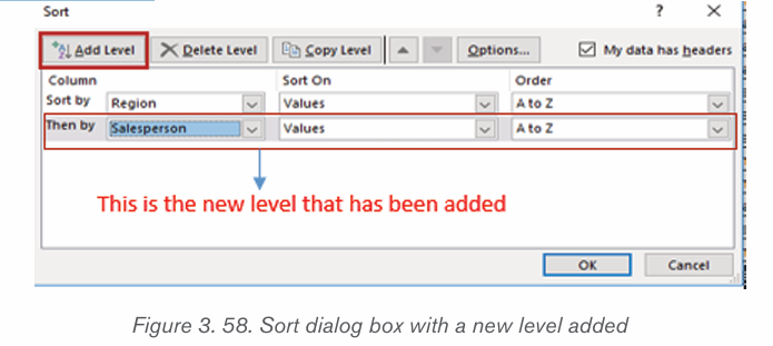 
Level instead of Add Level. In this case, you will only have to choose a different 
column in the first box.

 Step 5: Add more sort levels if needed, and click OK.

By sorting data by Region and then by Salesperson the data will be sorted first 

by the Region column then the second condition will be by Salesperson.

 Excel sort data in the specified order. As shown in the screenshot above,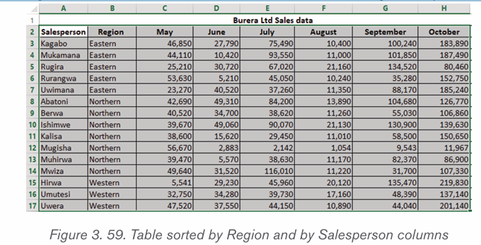 
data is arranged alphabetically exactly as it should: first by Region, and then 

by Salesperson

 3.8. Financial functions 

Application activity 3.8

1.Study the following table and answer the related questions:

 ii) Display the list of Items by ascending order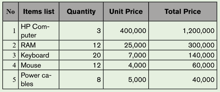
 iii) Print the Total price by descending order

 iv) Filter the items whose quantity is 12

Financial functions refer to the functions used to calculate financial information, 
such as net present value, future value and payments. For example, you can 

calculate the monthly payments required to buy a car at a certain loan rate.

3.8.1 The Net Present Value (NPV) Function
 Net present value (NPV) is the difference between the present value of cash 
inflows and the present value of cash outflows over a period of time. NPV is 
used in capital budgeting and investment planning to analyze the profitability of 

a projected investment or project.

 The NPV Function as an Excel Financial function will calculate the Net Present 
Value (NPV) for a series of cash flows and a given discount rate. It is important 
to understand the Time Value of Money, which is a foundational building block 

of various Financial Valuation methods.

The calculation of the NPV requires the identification of the number of periods. 
For example if there is a monthly cash flow for 5 years, there are 60 cash flows 

and 60 periods. It also requires to identify the discount rate .

The syntax of NPV Function is:
 =NPV(rate,value,[value2],…)
 The NPV function uses the following arguments:
 1. Rate (required argument) : This is the rate of discount over the length of 
the period.
 2. Value1, Value2 : Value1 is a required option. They are numeric values 
that represent a series of payments and income where:
 • Negative payments represent outgoing payments.
 • Positive payments represent incoming payments.

 For the example below the required rate of return is 10%. To calculate the NPV, 

use the formula and press enter key to get a result

The NPV formula is based on future cash flows. If the first cash flow occurs at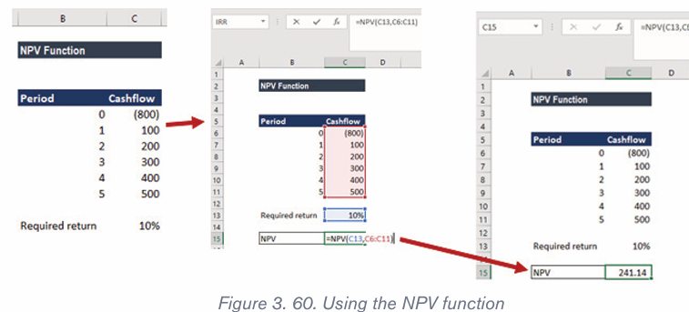 
the start of the first period, the first value must be added to the NPV result, not 

included in the values arguments.

3.8.2 The Future Value (FV) Function
 Value of the money doesn’t remain the same; it decreases or increases because 
of the interest rates and the state of inflation, deflation which makes the value of 
the money less valuable or more valuable in future. But for financial planning of 
what we expect the money for our future goals, we calculate the future value of 

the money by using an appropriate rate in a future formula.

 The Future Value formula gives the future value of money for the principle or 

cash flow at given period.

 FV is the Future Value of the sum, PV is the Present Value of the sum, r is the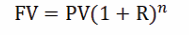 

rate taken for calculation by factoring everything in it, n is the number of years

Example of Future Value Formula

 In order to have a better understanding of the concept, calculate the future 
value by using the above-mentioned formula.

 Calculate the future value of 15,000,000 Rwf loaned at the rate of 12 
percent per annum for 10 years.

 To calculate the future value,

PV =15,000,000, R = 12 %, N= 10

 FV = PV (1+R)n, FV = 15000000 (1 + 0.12)10, FV = 46587720

Here the Present Value used is 15000,000, a rate of the period which is in years 

as 0.12, the number of periods which is year 10 years.

 Here 1.12 rate is raised to power 10, which is in years multiplied by the principle 

15000,000.

 It is very much used in each and every aspect of finance, whether it’s investments, 
corporate finance, personal finance, accounting etc.
 
The future Value of an investment depends on purchasing power it will be having 
and the return of investments on the capital.
 
Now, this cumulative of inflation and investment return is factorized in one term 

as the rate of return for the period.

Therefore,

 FUTURE VALUE = PRESENT VALUE + INCURRED RETURN ON 

INVESTMENT

Now to calculate this future value, we need to understand the value calculated 
will be used with a compounded rate of return over the years on the present 

value of the capital.

This can be explained by the example below:
 10 percent interest and capital is 1000, so the Future Value will be 1100 
equivalent to 1000+ 100. To calculate for 2 years, we can calculate by using 
1100 + 110 = 1210 which can also be written as 1000 (1.1) ^2 which will 
make the calculation to 1.21 * 1000 = 1210
 
This way, calculate the future values of any amount when an interest rate is 
given by the formula PV x (1 + r)ⁿ

 The calculation of Future Value in Excel is very easy and can take many variables, 

which can be very difficult to calculate otherwise without a spreadsheet.

The syntax of FV function:

 =FV(rate, nper, pmt,[ PV])

 Example: What will the amount after the principle of 10000 is invested 
for 10 years and 1000 is invested every year at the rate of 17 percent 

per annum.

Now, as soon as you put in the FV function and start a bracket, the excel asks you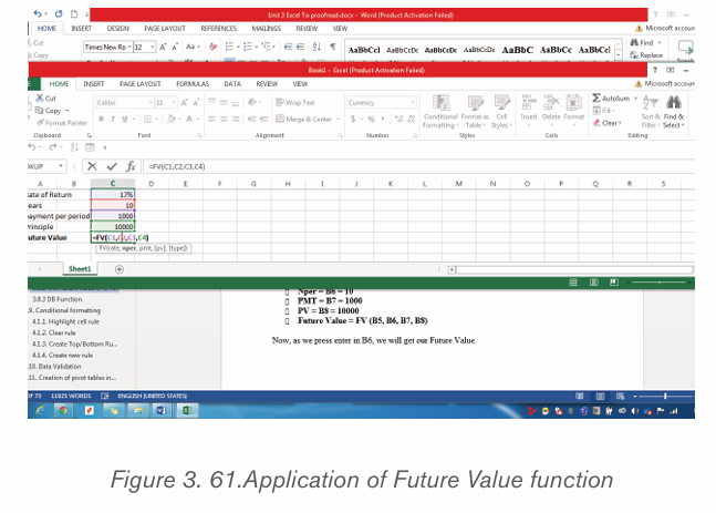 
to open the bracket and give rate (rate), a number of periods (nper), payment 
per term (pmt), Present Value (PV) close brackets.

 Now following the problem above: Rate = B5 = 17%, Nper = B6 = 10, PMT 
= B7 = 1000, PV = B8 = 10000

 Future Value = FV (B5, B6, B7, B8)

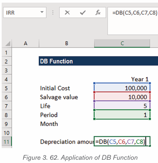
3.8.3. DB Function

The DB function is an Excel Financial function which helps in calculating the 
depreciation of an asset. The method used for calculating depreciation is 

the Fixed Declining Balance Method for each period of the asset’s lifetime.

 The syntax of DB Function:

=DB(cost, salvage, life, period, [month])
 • Cost (required argument): This is the initial cost of the asset.
 • Salvage (required argument): The value of the asset at the end of the 
depreciation.
 • Life (required argument): This is the useful life of the asset or the 
number of periods for which we will be depreciating the asset.
 • Period (required argument): The period for which we wish to calculate 
the depreciation for.
 • Month (optional argument): Specifies how many months 
of the year are used in the calculation of the first period of 

depreciation. If omitted, the function will take the default value of 

Activity 3.9

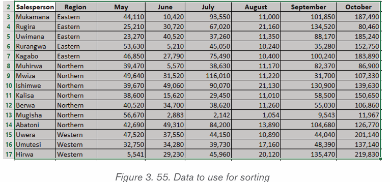
Open Excel and enter data in the table below. Save the File as “Burera Ltd Sales data”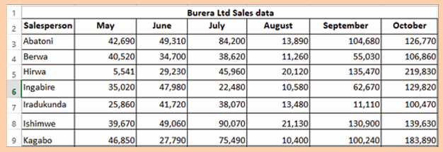


Do the followings:
 3. Using Burera Ltd Sales data, show salespersons who 
are meeting their monthly sales goals. The sales goal is 

50,000 items per month

4.Highlight all salesperson whose sales are below the average.
5.Highlight with blue color all salesperson whose sales are above 

6.80,000

 DB Function in Excel
 Example 1:
 Assume we wish to calculate the depreciation for an asset with an initial cost 
of 100,000 Rwf. The asset’s salvage value after 5 years is 10,000 Rwf. The 
screedshot below shows how to calculate it. The results are got after hitting the 

Enter key:

Application activity 3.8

 1.Explain all necessary arguments used by DB function
 2. What will the amount be (Future Value) after the principle of 
2500000 Rwf is invested for 8 years and 15000 is invested every 

year thereafter at the rate of 14 percent?

 3.9. Conditional formatting 

Conditional formatting is an especial feature (formatting feature) of Excel used to 
find unique and duplicates values by formatting the cells. Conditional formatting 
allows the users to format the cells and their data based on some conditions 
specified by the user. Using conditional formatting, you can highlight a cell with 

a certain color and its content with different font.

Conditional formatting enables spreadsheet users to do a number of things. 
First and foremost, it calls attention to important data points such as deadlines, 
at-risk tasks. It can also make large data sets more digestible by breaking up 
the wall of numbers with a visual organizational component. Among the options 
provided by conditional formatting are: highlight cell rules, top bottom 

rules, customized rules, etc

3.9.1. Highlight cell rule
Conditional formatting can be used to enhance the reports and dashboards 
in Excel. The conditional formatting statement under the Highlight Cells Rules 
category allow to highlight the cells whose values meet a specific condition.
 
The benefit of a conditional formatting rule is that Excel automatically reevaluates 
the rule each time a cell is changed provided that cell has a conditional formatting 
rule applied to it. Those rules include: greater than, less than, equal to, between, 
text that contain, A Date occurring, duplicate values, …
 
Here are the steps to apply the highlight cell rule:
 Step 1: Select the desired cells on which to apply the conditional formatting rule
 Step 2: From the Home tab, click the Conditional Formatting command. 

A drop-down menu will appear.

Step 3: Hover the mouse over the desired conditional formatting type, and then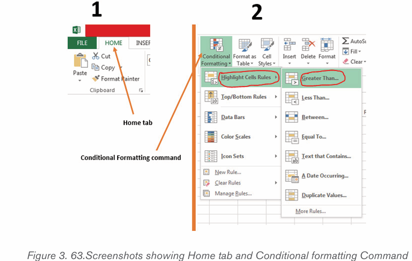 
select the desired rule from the menu that appears. In the Activity 4.1, we want 
to highlight cells that are greater than 50, 000.
 Step 4: A dialog box will appear. Enter the desired value(s) into the blank field. 
In the case of the activity 4.1.the taken value is 50, 000.
 Step 5: Select a formatting style from the drop-down menu. In the Activity 4.1, 

the color to choose is Green Fill with Dark Green Text, then click OK.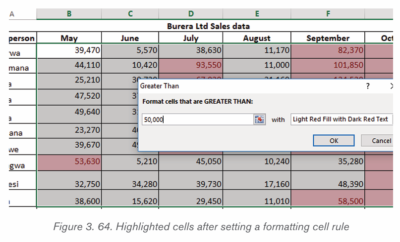

Step 6: The conditional formatting will be applied to the selected cells. In our 
case, it’s easy to see which salesperson reached the 50, 000 sales goals for 

each month.

 Note: You can apply multiple conditional formatting rules to a cell range or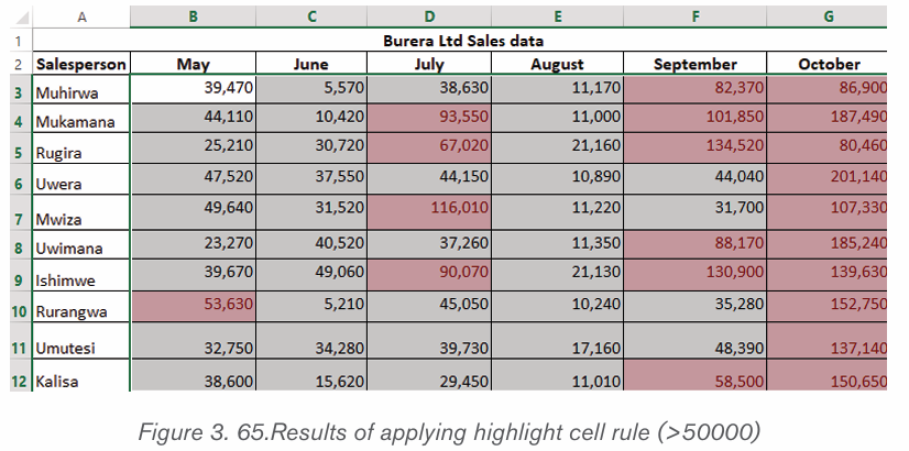 
worksheet, allowing you to visualize different trends and patterns in your data.
 
3.9.2. Clear rule
 Rules that have been used to highlight cells that meet certain conditions can be 
removed and have text with no highlight when the rules are no longer needed or 

when there is a need to set new rules. To clear rules do the following:

Step 1: Select the desired cells for clearing the conditional formatting rule
 Step 2: On the Home tab, in the Styles group, click Conditional Formatting 
(refer to Figure 4.1.)
 Step 3: Click Clear Rules then click Clear Rules from Selected Cells



 After clearing rules for selected cells, cells are no longer colored, there is no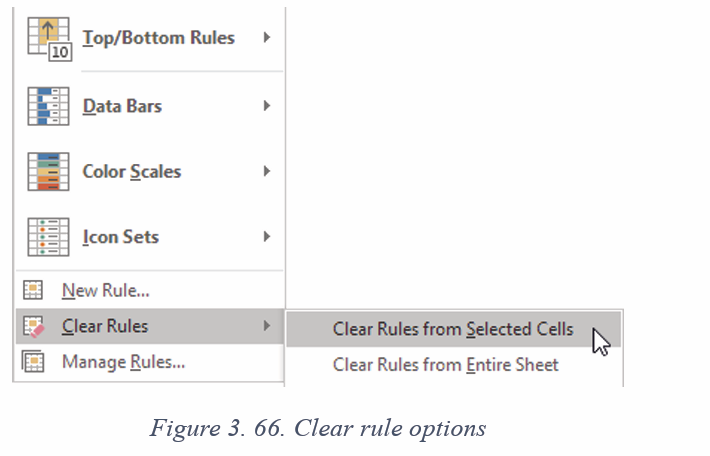 

more formatting in cells.

 3.9.3. Create Top/Bottom Rules
 Top/Bottom rules are another useful Conditional Formatting in Excel. These 
rules allow users to call attention to the top or bottom range of cells, which can 
be specified by number, percentage, or average.
 Step 1: Select the desired cells for the conditional formatting rule
 Step 2: From the Home tab, Select Conditional Formatting then Top/

 Bottom Rules then click Above Average…

 Step 3: A dialog box will appear. Choose color format to use like “Light Red Fill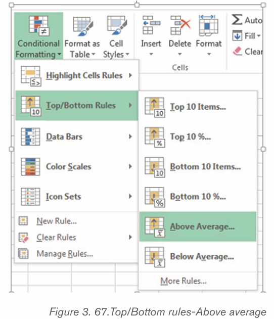 

with Dark Red text”. After choosing cells format, Press “OK”

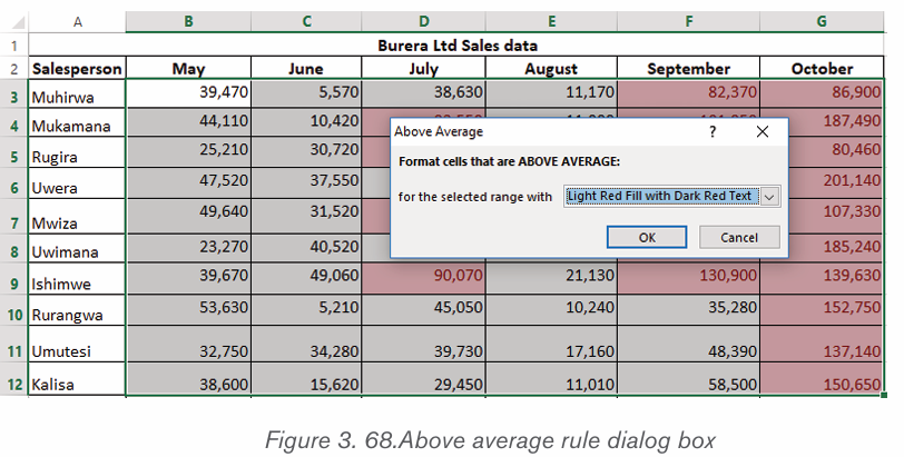
 Step 4: Your sheet will now highlight the values above the average 

 3.9.4. Create new rule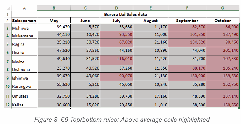 
Excel allows to create a formula-based conditional formatting rule. The available 
options are:
 • Formatting cells based on their values, 
• Formatting cells that contain certain values, 
• Formatting only top or bottom ranked values, 
• Formatting only values that are below or above average, 
• Formatting only unique or duplicate values and using a formula to 
determine which values to format. 

All those options are presented in the window below:

Step 1: Select the cells you want to format. In the Home tab click on Conditional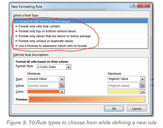 

Formatting command and click New rule

 Step 2: Create a conditional formatting rule, and select the Formula option then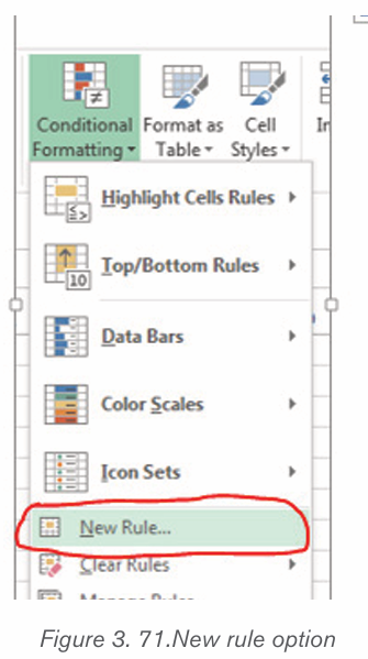 
click OK. In the window below the option “Use a formula to determine which 
cells to format” has been chosen
g) Format all cells based on their values
Step 1: New formatting rule window will be opened.
 Step 2: Select Format all cells based on their values option, however this is by 

default selected.

 In this case only 2 options are going to be used: 2-color scale and 3-color scale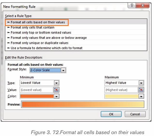
 h) 2-color scale 
Step 1: Choose minimum and maximum values

 Step 2: Click Ok button to apply this conditional formatting 

Step 3: Data set with this condition formatting will look like below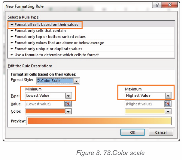
 Note: we have chosen minimum number to 50,000 and the maximum to 80,000, 

then selected a colors to separate both values.

 i) 3-color scale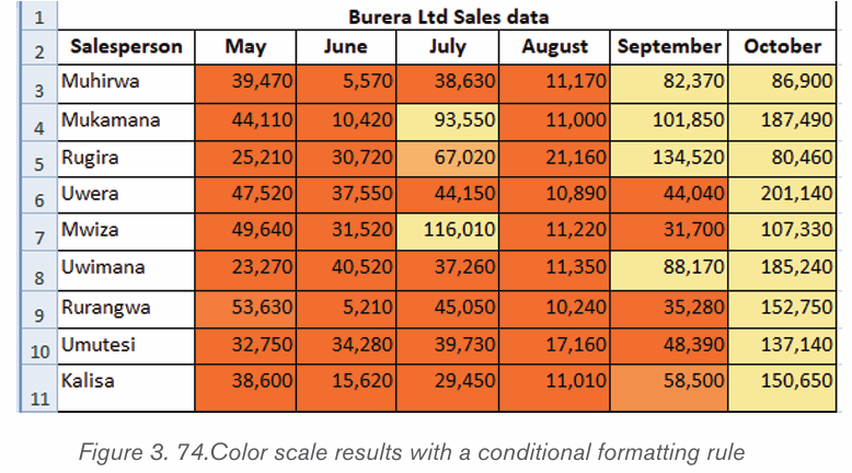
 Step 1: New formatting rule window will be opened.
 Step 2: Select Format all cells based on their values option, however this is by de

fault selected.

Below are steps to apply 3 -color formatting style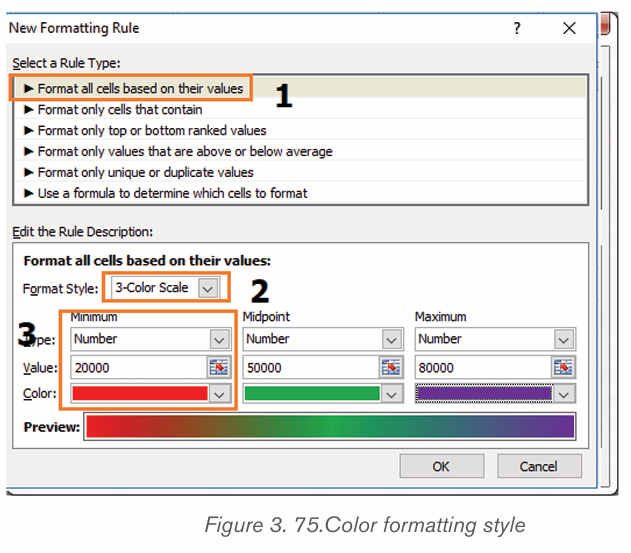
 Step 3: select 3 color scale option in format style 
Step 4: choose the type; here we are taking as Minimum, Midpoint and Maximum
 Step 5: Put values for number for Minimum, Midpoint and Maximum

 Then, results are displayed as follow: 

 2. Use a formula to determine which cells to format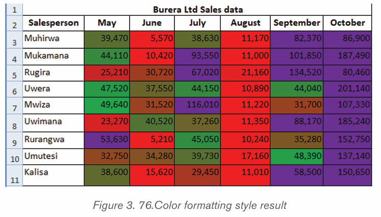
 New rules can be created by customizing own formulas. By using custom made 
formula, a custom condition that triggers a rule is created and can be applied as 
the user needs it to be applied. In the data that is going to be used the formula 
=B3>80000 has been applied for formatting.
 
To specify the formatting formula click on Conditional Formatting tab then New 
Rule and choose Use Formula to determine which cells to format as in the 

window below:

 Step 3: Enter a formula that returns TRUE or FALSE then set formatting options,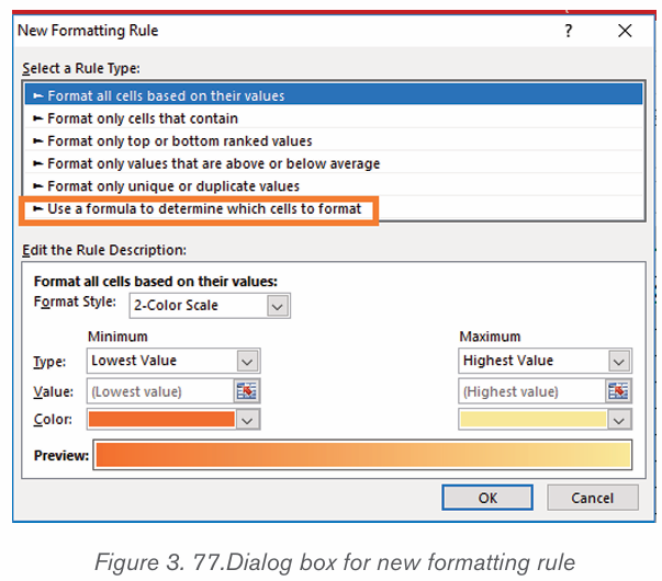 

save the rule and press OK

 After clicking OK cells that meet the formatting rule are highlighted as specified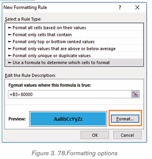 
in the new rule. In the window below cells meeting the criteria are blue colored 

as it has been specified.

 Note: Always write the formula for the upper-left cell in the selected range.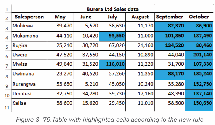 
Excel automatically copies the formula to the other cells. Thus, cell B3 contains 
the formula =B3>80,000, cell C3 contains the formula = B3>80,000 and etc.
 
Below are some formulas that apply conditional formatting and return TRUE or 
FALSE, or numeric equivalents.

 =ISODD (A1): The ISODD function is used to check if a numeric value is an 
odd number. ISODD returns TRUE when a numeric value is odd and FALSE 
when a numeric value is even. If value is not numeric, ISODD will return the 
#VALUE error.
 
SODD (A1) returns TRUE if A1 contains the number 3 and FALSE if A1 contains 
the number 4.Usually, value is supplied as a cell address.

ISODD is part of a group of functions called the IS functions that all return the 

logical values TRUE or FALSE.

1) =ISNUMBER (A1): The ISNUMBER function is used to check if a value 
is a number. ISNUMBER will return TRUE when value is numeric and 
FALSE when not.
 
2) ISNUMBER (A1) returns TRUE if A1 contains a number or a formula 
that returns a numeric value. If A1 contains text, ISNUMBER will return 
FALSE.

 3) AND (A1>100, B1<500): The AND function is used to apply more 
than one condition at the same time, up to 255 conditions. Each logical 
condition (logical1, logical2, etc.) must return TRUE Examples
 
4) AND (A1>100, B1<500) test if the value in A1 is greater than100 and 

B1 less than 500

Application activity 3.9

 • Given the following data tables :

1. Using conditional formatting highlight with red color the total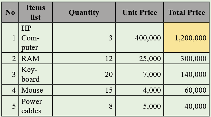 
prices which costed between 150,000 and 500,000
 2. Apply conditional formatting on Total price using data bars
 3. Apply conditional formatting on Unit price using Color scales

 4. Apply conditional formatting on Quantity using Icon sets

3.10. Data Validation

 Activity 3.10

  1.What do you understand by data validation ?
 2. What is the importance of applying data validation

Data Validation is one of the essential features in MS Excel. When creating an 
Excel sheet for users or customers, you may often need to restrict the inputs 
based on different criteria to ensure that all the entries or inputs are correct and 
consistent. Data Validation is the solution that helps to control user inputs into 

specific cells or a range according to the specified rules.

Some of the essential tasks (restrictions/ validations) that can be set using the 
Data Validation are as follows:

 • Allow users to put numeric or text entries only
 • Allow entering numbers less than, more than and between a 
specified range
 • Allow data inputs of a specific length
 • Restrict entries to predefined values in a drop-down list
 • Restrict date and time entries outside or within a specific range
 • Validate a specific entry based on another cell
 • Display an input message informing users what the corresponding 
cell accepts when the user selects a cell
 • Display a warning or error message when the user enters wrong data
 • Locate incorrect or wrong entries in the validated cells

 Applying Data Validation on any cell or range of cells in an Excel sheet restricts 
the users from entering any undesired entries in corresponding cells based on 
the validation rules. For instance, if we set validation to accept only numbers 
or numeric values, other users will not be able to enter any values other than 
numbers. The Excel data validation window is displayed after clicking on the 
Data tab then click on Data Validation. After the Data Validation window is 
available, choose among the different optins which are available by clicking on 

the Setting tab, Input Message tab, Error Alert tab.

 Data Validation can be configured to show an input message to users when the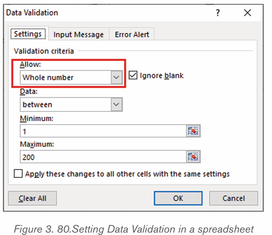 

respective cell is selected, informing them what is allowed in it, as shown below:

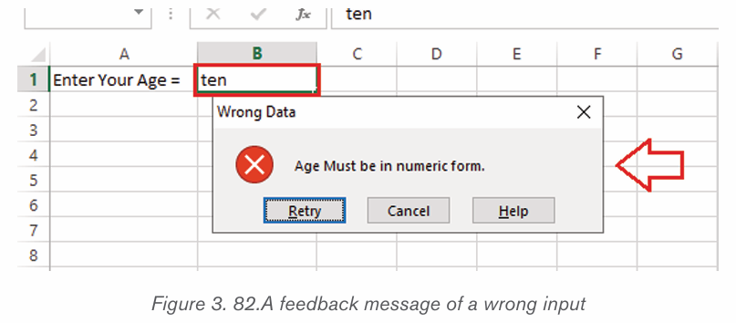
 As soon as we try to enter any other type of data in restricted cells, Excel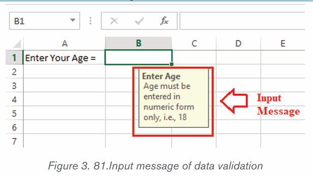 
instantly displays an error message and even can display which type of data 
the respective cells can accept. The error message can be of different styles 
and customized or created manually while setting up the validation rules on the 

Excel sheet.

 • Data Validation Controls

 The Data Validation feature or its controls can be found on the ribbon under the 
Data tab. By default, it is placed under the category ‘Data Tools’.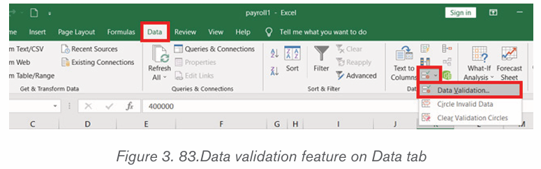

 As soon as Data Validation icon is clicked from the ribbon, it immediately 
launched a Data Validation dialog box. In addition to the Data Validation 
shortcut on the ribbon, the keyboard shortcut ‘Alt + D + L’ can be used without 
quotes. It will launch the Data Validation dialog box instantly.

 Using Data Validation Dialog Box to Define Validation Rules
 
The Data Validation dialogue box contains three essential options/ tabs: Settings, 
Input Message, and Error Alert.

• Settings Tab
 The settings tab provides us options to set validation criteria. The tab helps us 
choose the desired validation rules from the built-in options we want to allow 
in selected cells. Moreover, we can also set custom rules with the customized 
formula to validate user inputs. The settings tab contains all the data validation 

options present in Excel.

 • Input Message Tab
 The input message tab has a text box to enter a message displayed as soon 
as the respective cell is selected. The input message is an optional feature of 
Data Validation. If we do not define any message as an input message, excel 
does not show any message when the user selects the respective cell with data 
validation. It does not affect the working of the data validation and has no effect 
or control over what the user enters into a cell. However, it can be helpful to 

inform users about the allowed or expected data values.

 • Error Alert Tab
 The error alert tab provides options to control the way how the validation is 
enforced. We can set criteria and then use any desired error style to accept or 
reject the user inputs accordingly. Additionally, we can also display a message 
to the user informing what the error is or what values must be entered in 

corresponding cells.

 • Adding Data Validation in Excel
 Step 1: Launch the Data Validation dialogue Box
 To add a data validation in an Excel sheet, we must perform the following steps:

 First, select all the cells or a range to which to apply the validation. Next, ckick 
the Data tab. In the Data Tools group and select Data Validation tool to 

launch the data validation dialogue box.

 Step 2: Set the Data Validation Rule
 After the data validation dialogue box is displayed, go to the Settings tab to 
define validation criteria. Provide the desired values, cell references, or formulas 

in the validation criteria.

 After all the validation settings have been set, click the OK button to close the 
validation dialog box or move to the next tab to insert an input message and/or 

error alerts. 

Step 3: Create an Input Message to Display (Optional)
To display a message to the user saying which type of data is supported
or allowed in the selected cell, use the input message tab. Using the input 
message, the useris informed about the allowed data type format when the user 
selects corresponding cells.
 
Once the input message is entered, click the OK button or move to the Error 
Alert tab further.
 
Step 4: Add an Error alert (Optional)
 In addition to an input message, set an error alert to display when the user enters 
invalid data into the respective cells. Moreover, add a custom error message.

Application activity 3.6
 a.Apply the following data validations in the table below :
 1. If the age is not belonging the range of 60 and 75, error message
 2. If the Date of birth exceed 1960, provide an error message
 3. If the entered country is not RWANDA in UPPER CASE, prompt an 

error message

3.11. Pivot tables in Excel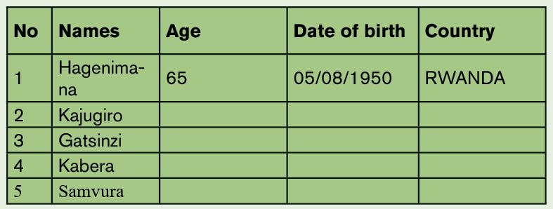
 Activity 3.11
 By doing a research using the  internet or any other resource 
answer the following questions
 1. What do you understand by a pivot table?
 2. Discuss the uses of a pivot table 
3. Outline different steps of creating a pivot table

A pivot table is a statistics tool that calculates, summarizes, analyzes and 
reorganizes selected columns and rows of data in a spreadsheet or database 
table to obtain a desired report. Pivot tables are especially useful with large 
amounts of data that would be time-consuming to calculate by hand.
 
• Uses of a pivot table
 • A pivot table helps users answer business questions with minimal effort. 
Common pivot table uses include:
 • To calculate sums or averages in business situations. For example, 
counting sales by department or region.
 • To show totals as a percentage of a whole. For example, comparing 
sales for a specific product to total sales.
 • To generate a list of unique values. For example, showing which states 
or countries have ordered a product.
 • To create a 2x2 table summary of a complex report.
 • To identify the maximum and minimum values of a dataset.
 • Creating a pivot table in Excel
 • Select the cells you want to create a PivotTable from. 

• Click Insert tab and then PivotTable.

• Choose where you want the pivot table report to be placed. Select New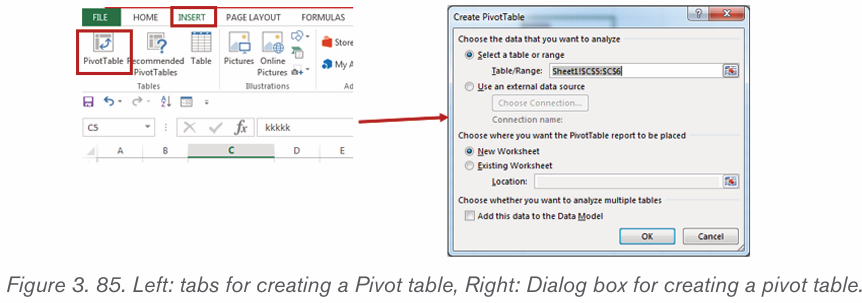 
Worksheet to place the pivot table in a new worksheet or Existing 
Worksheet and select where the new PivotTable will appear.
 • Click OK.
 • Choose the fields to add to a report on right pane of the window
 • Drag fields between areas below:
 • Performing the steps of creating a pivot table 

Go through these steps to create a pivot table:
 Step1: Select the cells on which to create a PivotTable and click Insert tab 

and then select PivotTable.

 Step2: This will create a PivotTable based on an existing table or range. By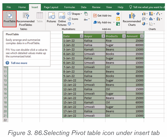 

clicking Pivot table tool  the Create PivotTable dialog box appears

Step 3: Choose where the PivotTable report will be placed. Select New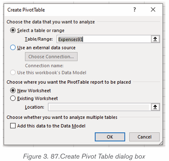 
Worksheet to place the PivotTable in a new worksheet or Existing Worksheet and 
select where the new PivotTable will appear.
 Step 4: Click OK.
 Step 5: Choose the fields to add to a report on right pane of the window

 Step 6: To obtain a report result, drag product and date filds to values area 

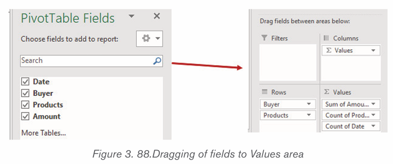
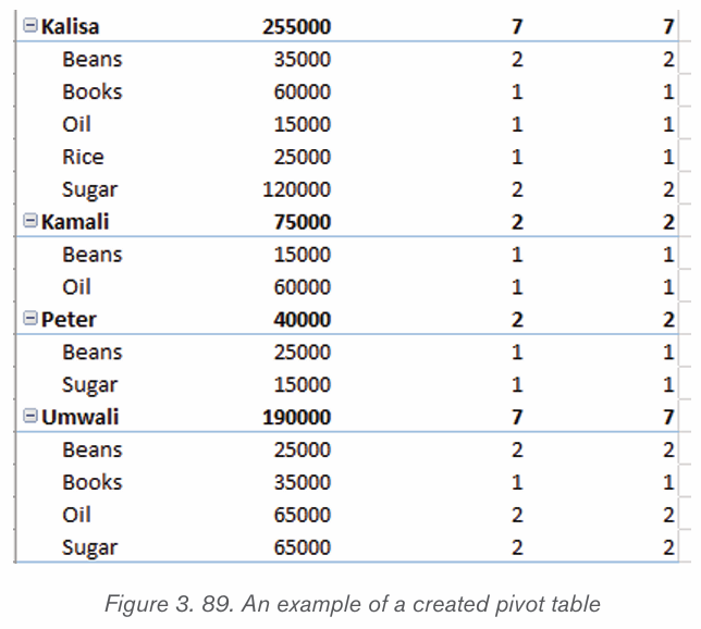
After dragging the fields needed, a pivot table is created automatically as follows:

Application activity 3.11

 1. You have a list of all students of your class. The list contains the 
gender of each student and the district where he/she came from. 
You are requested to do the following:
 • Separate the list in different sheets, sheet 1 contains the male students 
and sheet 2 contains the female students.

 • Show the number of students by the district where they come from.

3.12. Excel data entry forms
 Activity 3.12
 1 What do you understand by data entry form?
 2.  Using internet search, discuss the process of creating Excel 

data entry forms?

 Excel offers the ability to make data entry easier by using a form, which is a 
dialog box with the fields for one record. The form allows data entry, a search 
function for existing entries, and the ability to edit or delete the data.

 The example below has two fields per record. The form allows up to 32 fields 

per record.

 Here below are steps to be performed while creating an Excel data entry form: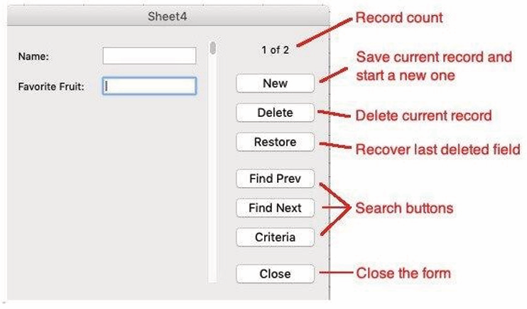
 Step 1: On the chosen sheet, highlight the number of columns needed.
 Step 2: Click insert tab and then click table icon
 Step 3: In create table dialog box, select My table has headers checkbox and 

click Ok

Step 4: Change the default column headers, and adjust the width of columns if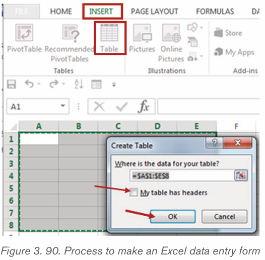 

necessary.

 Step 5: Click Form Icon of Customize Quick Access Toolbar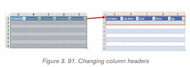
 Step 6: The form will appear. The number of columns in the table will match the 
number of fields on the form. The column titles in the table will be the field titles 

on the form. You are now ready to enter data records into the form.

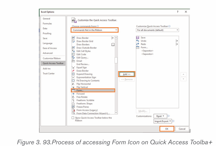
Note that Form Icon is accessed by performing the following steps: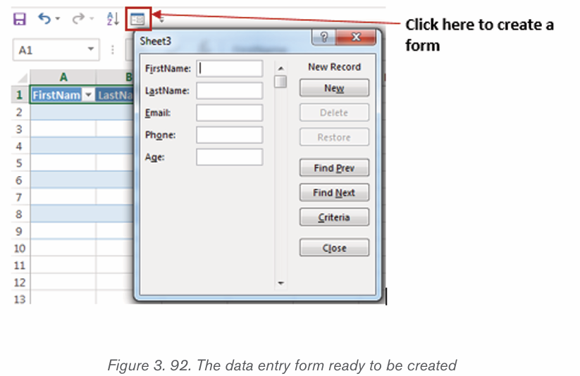
 Step1: On Customize Quick Access Toolbar , click More Commands option
 Step2: Select Commands Not in the Ribbon and then select Form icon
 Step3: Select Add Button

 Step 4: Click Ok Button

Application activity 3.12

Study the following Excel data entry form and create it:

Skills lab 2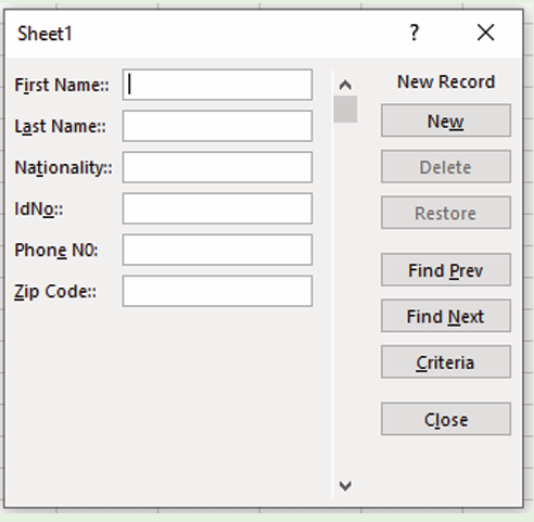
 The school organizes an event to welcome new students. All expenses of the 
event will be covered by the school. You are requested to prepare a budget of 
an event in your class S4. The budget must be done in Ms Excel spreadsheet 
with the following:
 Use Excel formulas and functions to do different calculations, also use different 

table styles to make the budget more understandable.

End of unit assessment 3

Q1. Explain the following terms:
 a. Loan amortization
 b. Data Validation
 Q2. Discuss any two financial functions and write their general formats 
(syntaxes).
 Q3. Discuss any four uses of a pivot table
 Q4. Outline different steps of applying conditional formatting using data bars
 Q5. On 2nd January, Kamali invested 1,000,000 Rwf in a saving account of 
his BPR account at 8% annual interest rate. Calculate the amount of his 
savings at the end of year?
 Q6. On 10th July 2019, Mukamana took a loan of 3,000,000 Rwf from 
Umurenge SACCO.
 You are requested to calculate and show the whole process of 
reimbursement of Mukamana’s loan from August 2019 to August 2022 at 

the interest rate of 18%